2020년 3월 29일 일요일

COVID-19, 분자생물학으로 바라보기

최근 블로그에서 COVID-19가 경제와 사업에 미친 영향들에 대해 조금 다뤄봤는데, 오늘은 분자생물학적 관점으로 바라본다.


코로나 바이러스 기본 정보부터 알아보자.


먼저 COVID-19(coronavirus disease 19)는 병명이고, 이를 일으키는 바이러스가 신종 코로나인데 바이러스의 정식 명칭은 SARS-CoV-2이다. SARS는 우리가 아는 사스이고 풀어 적으면 severe acute respiratory syndrome, 즉, 중증 급성 호흡기 증후군이다. 2002, 2003년 사스 바이러스(SARS-CoV)의 사촌격이다. CoV는 코로나바이러스 줄임말이다. 

코로나바이러스는 단일가닥 RNA 바이러스다. 바이러스를 분류하는 방법은 여러 가지가 있지만 유전정보를 DNA에 담느냐 RNA에 담느냐에 따라 나눌 수도 있다. 대표적인 DNA 바이러스로 헤르페스(herpesvirus)가 있고, 에이즈를 일으키는 HIV는 코로나처럼 단일가닥 RNA 바이러스다. RNA는 원래 단일가닥이지만 이중가닥 RNA로 보관하는 바이러스도 있는데 로타바이러스가 대표적이다. 

코로나로 돌아오면, 박쥐가 대표적이지만 이외에도 다양한 척추동물을 감염시킨다. 돼지와 소에서 장염을 일으키며, 닭에서 호흡기 질환을 일으킨다. 사람에게서도 익숙하다. 겨울철에 흔히 걸리는 일반 감기의 원인 바이러스 중 하나이기 때문이다. 다만 SARS-CoV들은 보통 박쥐로부터 유래하고 유전적으로 일반 감기 코로나와는 다른 특징을 보인다. 


이번 코로나는 기존 코로나랑 유전적으로 어떻게 다른가?


중국 우한시에서 사태가 발발한 이후 즉각적으로 Chinese Academy of Sciences와 우한의 한 병원팀이 함께 Nature에 논문을 발표했다(Zhou et al., 2020). 즉시 중국 내 7명의 환자로부터 샘플을 확보했고, 이를 가지고 유전분석을 진행한 것이다. 유전체 시퀀싱을 위해 pan-CoV PCR 프라이머를 사용했는데, 지난 사스 때 사용되었던 프라이머다. 7개 샘플 중 5개에서 CoV가 검출되었다. 이중 하나로 메타지노믹스 분석에 들어갔다. 10,038,758개의 total reads를 확보했고, 이중 인간 유전체로부터 온 것을 제외하면 총 1,582개의 reads였다. 이중 87.1%인 1,378개가 SARS-CoV와 일치했다(아래 그림). 결국 SARS-CoV와 같은 놈이거나 적어도 친적이겠다. 


같은 녀석일까 새로운 녀석일까. 총 서열을 합친 결과 이번 SARS-CoV-2는 총 29,891의 염기서열로 이루어진 유전체를 가지고 있었다. 이중 79.6%만이 2002년 사스 때의 바이러스인 SARS-CoV와 일치했다. 같은 종이지만, 유의미한 차이가 보인다. 환자 샘플별 상동성은 99.9%에 달했으므로, 이 녀석이 바로 이번 사태를 일으킨 신종 코로나 바이러스다. 단백질 레벨로 가면 그래도 아미노산 서열이 SARS-CoV와 94.4% 상동성을 보인다고 한다. 즉, 신종이긴 하지만 사스 그 녀석과 같은 종임을 다시 한번 알려준다.


같은 듯 다른 듯. 전체 코로나 중 어디에 위치하며 누구와 유사한지에 알아보려면 계통수를 그리는 것이 확실하다. 연구팀은 코로나의 유전자 중 RNA-dependent RNA polymerase (RdRp)와 spike (S) 서열로 계통수를 그렸다(뒤에서 다루겠지만 spike가 인체 감염의 핵심 단백질이다). 위의 계통수에서 볼 수 있듯 코로나의 종류가 상당히 많은데, 연구팀이 중국 환자 샘플에서 얻은 바이러스(빨간 상자)는 확실히 사스 녀석들과 비슷하지만 다른 곳에 위치하고 있다. 이번 코로나 바이러스의 근원지로 추정되는 중국 원난성의 중간관박쥐(Rhinolophus sinicus)로부터 확보한 바이러스(Bat CoV RaTG13)와 가장 유사함을 알 수 있다. 역시 박쥐에서 유래했던 것이다.

이번 코로나가 기존 사스 코로나와 주목할 만한 차이가 나는 부분은 바로 spike 단백질이다. Spike 단백질은 인체 감염에서 핵심적인 역할은 한다. SARS-CoV의 spike 단백질은 S1과 S2의 subunit으로 구성되어 있는데, S1은 인간세포 수용체와의 결합에, S2는 결합 후 세포막 퓨전에 역할을 한다. 기본적으로는 유사할 테지만 SARS-CoV-2와 SARS-CoV 간의 spike 단백질 상동성은 75% 밖에 되지 않는다. 일단 이번 코로나의 spike 단백질이 길다. 그리고 N 터미널에 3개의 짧은 삽입이 발견되며, 수용체 결합 부위의 핵심 서열 5개 중 4개가 다르다고 한다. 이런 차이가 어떤 의미가 있는지는 더 연구해 봐야 알겠지만, spike 단백질이 인간세포 감염에 관련되어 있기 때문에 이 차이가 높은 감염성과 전염성에 기여하는 부분이 아닐까 한다.


그럼 인간을 감염시키는 분자생물학적 기작은 무엇일까?


인간 폐 세포에는 angiotensin converting enzyme II (ACE2)라는 단백질이 존재는데, 2002년 사스 코로나인 SARS-CoV는 ACE2를 통해 인간 세포 내로 진입함이 알려져있다. 위의 논문으로 이야기를 이어 나가자면, 연구팀은 이번 코로나인 SARS-CoV-2도 ACE2를 통해 감염하는지 확인해 보고자 했다. HeLa 세포에 다양한 동물의 ACE2를 발현시킨 후 SARS-CoV-2가 세포로 들어갈 수 있는지 확인하는 것이다. 인간, 박쥐, 돼지, 고양이, 마우스의 ACE2를 시험한 결과 마우스 ACE2 발현 세포를 제외하고는 전부 코로나로 감염되었다(아래 그림). ACE2를 발현시키지 않은 대조군(control)에서는 바이러스 감염이 관찰되지 않았다. 이로써 ACE2가 SARS-CoV-2의 감염 경로임을 강하게 시사한다. 연구팀은 다른 코로나의 감염 경로로 알려진 다른 수용체로도 시험해봤는데, SARS-CoV-2는 aminopeptidase N (APN)이나 dipeptidyl peptidase 4 (DPP4)를 통한 감염은 못한다고 한다.


그럼 ACE2를 통해 들어가는 기작은 뭘까? 먼저 2002년 사스 바이러스의 기작을 살펴보자. 2013년 독일 연구팀이 발표한 논문에서 단서를 찾아본다(Heurich et al., 2013). SARS-CoV가 세포 내로 진입하려면 spike 단백질이 인간 세포의 ACE2와 결합을 해야한다. SARS-CoV의 spike 단백질의 S1 부위는 ACE2와의 결합에, S2 부위는 결합 후 세포막 퓨전에 역할을 한다고 했다. 일단 ACE2와 결합하면 spike 단백질의 구조가 변형되고, S1과 S2를 이어주는 부분이 잘리게 된다. 이 'cleavage'가 감염을 위해서는 꼭 필요하다. 그런데 이걸 자르는 효소는 바이러스의 것이 아니라 숙주, 즉 인간의 것이다. 알려진 효소는 cathepsin L과 type II transmembrane serine proteases (TTSPs)가 있다. Cathepsin L은 바이러스가 숙주세포의 엔도좀으로 들어오면 잘라주는 pH-dependent endo-/lysosomal protease다. TTSPs로는 TMPRSS2와 HAT이 알려져 있는데, 이들은 엔도좀이 아닌 숙주세포막에서 잘라주는 효소다. Cathepsin L 경로와는 독립적인 경로다. TMPRSS2와 HAT 모두 ACE2가 발현되는 폐 세포에서 발현된다. 기존 연구결과들을 보면 TMPRSS2가 SARS-CoV 감염에 중요한 역할을 한다고 한다. 독일 연구팀의 논문에서는 이 효소가 spike 단백질뿐만 아니라 ACE2도 잘라주며, 이 과정이 감염에 필수적임을 밝혔다. 또한 ACE2의 697번에서 716번 아미노산 중 알지닌과 라이신이 이 절단에 필요함을 알아냈다. 그리고 다른 효소인 ADAM17도 ACE2 절단에 관여는 하지만 이는 코로나의 감염과는 무관함을 밝혔다. 이를 도식화한 것이 아래 그림이다.


그럼 이번 SARS-CoV-2도 감염을 위해 TMPRSS2를 필요로 할까? 답은 YES이고, 마침 같은 독일팀이 이를 밝힌 결과를 최근 Cell에 발표했다(Hoffmann et al., 2020). 바이러스만 바꼈을 뿐 내용은 2013년 논문과 별반 다르지 않을 것이다. 아래 그림이 요약이다.


결국 ACE2와의 결합, TMPRSS2의 보조를 통해 SARS-CoV-2는 인간 세포에 들어온다.


그러면 COVID-19의 증상은 어떻게 설명할 수 있을까?


그러면 이번 SARS-CoV-2에 감염되면 왜 호흡기 증상을 보이고, 또 1% 정도의 치사율까지 보이는 것일까. 이는 마침 페친 한분께서 관련 유튜브 내용을 공유해주셔서 쉽게 정리할 수 있었다. 이 영상이 마음에 드는 점은 코로나의 '감염성'과 '유독성'을 분명히 구분해서 설명한다는 것이다. 주변이나 언론에서 이 개념을 혼동해서 쓰는 경우가 많다.


그림이 조금 복잡하지만, 4사분면으로 나눠서 설명해보겠다. 

  1. 좌상단: 인간 폐에서 발현되는 ACE 단백질이다. 이제껏 ACE2를 설명해왔는데, ACE1이 드디어 나타났다. 일단 ACE-angiotensin converting enzyme-는 그 이름에서 알 수 있듯 혈관수축에 관여하는 효소이다. ACE1와 ACE2는 서로 길항작용을 하는데, 각각 혈압상승과 강하에 기능을 한다. 더불어 ACE2는 면역완화에도 역할을 한다. 옆에 spike 단백질과 ACE2의 결합 구조도 살짝 보인다. 
  2. 우상단: 최근 Lancet에 실린 기고문인데, 고혈압과 당뇨에 걸린 사람이 COVID-19 감염 확률이 높을까라는 제목이다. 답은 그렇다이고 아래 설명한다.
  3. 좌하단: '감염성'에 대한 설명이다. 고혈압, 당뇨, 심혈관질환 환자는 혈압을 낮추기 위해 ACE1 억제제(ACEi)를 복용한다. 이는 오히려 ACE2의 수를 증가시키는 역할을 한다고 하는데, 영상에서는 충분히 설명되지 않아 Lancet 기고문을 찾아봤다. ACE2의 발현은 ACEi와 angiotensin II type-I receptor blockers (ARBs)를 투여한 당뇨환자에게서 올라간다고 한다. 고혈압 환자도 마찬가지. 그리고 치아졸리딘디온(thiazolidinediones, 혈당관리약물)이나 이부프로펜(!)에 의해서도 ACE2의 발현이 올라간다고 한다. 정리하자면, 당뇨나 고혈압과 같은 질병 자체보다는 이 환자들이 투여하는 약물로 인해 ACE2의 발현이 높아지고, ACE2는 코로나의 감염 경로이기 때문에, 결국 SARS-CoV나 SARS-CoV-2의 감염 확률이 높아지는 것이다.
  4. 우하단: '유독성'에 대한 설명이다. 코로나가 ACE2와 결합해서 세포 안으로 들어갈 때 ACE2를 끌고 들어간다고 한다. 이때문에 폐 세포 표면의 ACE2의 수가 줄어들게 되고, 이는 혈압강하와 면역완화의 기능이 떨어짐을, 즉, 혈압이 오르고 염증반응이 발생함을 의미한다. 더 심각한 것은 폐와 관련되어 있다. ACE2는 폐에서도 특히 폐포의 type 2 pneumocyte에 위치하는데 이 세포는 계면활성제를 분비하여 폐포가 팽창한 형태로 유지될 수 있게 한다. 이런 용적이 확보 되어야만 가스교환이 원활하게 일어나고 우리가 충분한 산소를 얻을 수 있다. 하지만 ACE2가 줄어들면 이 가스교환, 즉, 호흡에 문제가 생긴다. 그리고 염증 과민반응으로 인해 폐 세포의 섬유화가 진행된다. 호흡기 증상이 바로 이런 이유에 기인한다.

ACE2가 역시 모든 설명의 중심에 있는데, 결국 ACE2가 많으면 '감염성'이 높아지고, 감염 후 ACE2가 줄어들면 '유독성'이 높아진다. 많아도 문제, 줄어도 문제(앞에서 이부프로펜이 ACE2 발현을 올려 감염성이 높아진다고 했는데, 일단 감염되고 나면 오히려 이부프로펜을 많이 먹어야 하는 것 아닌가?). 현재 제약업계에서는 COVID-19의 치료제로 ACE2 항체도 개발 중인 것으로 알고 있는데(항체가 코로나 대신 ACE2와 결합하여 코로나 감염 방해), 이 항체가 ACE2의 역할에 지장을 주면 부작용이 클 수 있겠다는 생각이 든다. 결국 코로나도 바이러스 자체가 위험하다기 보다는 바이러스가 ACE2의 숫자를 줄이는데 기여를 하므로 위험한 것인데, 항체가 오히려 그 위험을 근본적으로 촉발시킬 수 있는 역설적인 상황이 될 수도.

이 영상에서는 기타 FAQ에 대한 대답도 잘 설명해준다. 왜 나이 많으신 분들이 더 심각할까, 왜 남자가 더 감염되기 쉬운가 등. 


이상 작금의 사태에 대해 분자생물학적인 관점으로 정리해봤다. 

정확하게 알아야 제대로 대처할 수 있다. 인간에게서 감정을 빼앗으면 황폐함만 남는다. 하지만 지금은 감정이 지나치게 과학을 앞서 나가면 안되는 시점이다.

* 페이스북 링크: https://www.facebook.com/820850277/posts/10159478214090278/?d=n

2020년 3월 17일 화요일

COVID-19와 주식시장 (as of 3/17/2020)

신종 코로나로 인해 주식시장에 곰의 울부짖음이 심하다. 주변의 반응을 살펴보면 이렇다.


  1. 곧 회복될 시장이다 (Investments 수업 대부분의 학생들 및 교수님)
  2. 10년 주기 불황이 드디어 왔다 (여의도 증권가의 많은 이들)
  3. 모르겠고 무섭다 

나는 1번이라고 믿고 있지만 생각보다 회복이 더딘 게 -오히려 하락이 지속되는 게- 현실이라 불안하기도 하다. 앞선 글에서 회복을 믿는 이유를 몇 가지 늘어놨지만, 불황, 혹은 꼭 불황까지는 아니더라도 조정을 예상하는 글들이 있어 정리해본다. 

먼저 Barron's에 2월 21일자로 실린 "Stocks Drop on the Week but Still Look Bubbly. Time to Prepare for a Correction."라는 제목의 기사다. 핵심 문단만 뽑아봤다.


It is what’s going on under the surface that looks worrisome. Growth stocks are dominating value stocks, blowing past dot-com-era outperformance levels. “The last time we got to these levels, the bubble burst and a 50%-plus global bear market began,” Citigroup strategist Robert Buckland pointed out in a Friday research report.

Consider the trading action in the market’s most popular stocks. The FAANGs— Facebook (ticker: FB), Apple (AAPL), Amazon.com (AMZN), Netflix (NFLX), and Google parent Alphabet (GOOGL)—are up 10% year to date, adding more than $330 billion in market value to the S&P 500. What’s more, the average price/earnings ratio for FAANG stocks has jumped to 35 times estimated earnings from 21 times last year.

버블론. Value 주에 비해 growth 주가 최근 너무 힘을 받고 있고 P/E ratio도 너무 높다는 주장. 닷컴 버블 때와 비교하며 상당히 비판적으로 시장을 보고 있다. 일리 있는 주장이다. 이 주장은 작년부터 계속 존재했었다. 특히 미국 국채 장단기 금리가 역전 되면서 불황이 현실화 된다고 말하며 위와 같은 주장이 근거로 등장하곤 했다.

물론 이에 대한 반박의 논지도 있다. 먼저 닷컴 때와 다르게 FAANG 주들은 현재 탄탄한 매출과 현금흐름이 뒷받침 되고 있기 때문에 허상이 아니라는 주장. 그리고 전체 시장의 P/E가 높아 보이지만 실제로는 FAANG의 시총이 20% 가까이 차지하기 때문에 나머지 주들의 P/E는 그리 높지 않다는, 즉 전체 시장 버블은 없다라는 논지다.

두 주장 모두 일리가 있고, 또한 어느 한 방향으로 흘러간다고 해서 다른 주장이 틀렸다고 말하기도 어렵다. 현실은 너무 많은 요인들에 의해 결정되기 때문에 그 누구도 모른다.

어제 The Wall Street Journal에 재미있는 기사가 났다. "Why Are Markets So Volatile? It’s Not Just the Coronavirus."라는 제목의 기사인데, 코로나 이면의 시장변동성이라고 하길래 나는 경기 불황을 WSJ에서 드디어 다룬다고 생각하고 읽었지만 그런 내용은 아니었다. 상당히 긴 글인데, 내가 이해한 요지는 많은 기관투자자는 요즘에는 컴퓨터 프로그래밍에 의한 투자를 진행하고, 이 프로그램에서 투자를 결정하는 중요한 요인이 바로 변동성(volatility, 즉 risk와 동일한 의미이다)이라는 것이다.

stock variance formula 이미지 검색결과

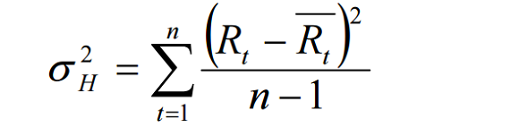
변동성은 표준편차다. 위의 식은 이를 제곱한 분산(variance)를 구하는 식이다(과거데이타로 구하고자 할때). 그냥 우리가 아는 분산식이다. Rt는 t라는 시점의 수익률이고, Rt bar는 우리가 측정하고자 하는 기간 동안의 수익률 평균이다. 분모의 n-1은 그냥 n이라고 생각해도 된다(통계상 자유도랑 관련된 것). n은 수집한 데이터의 수이다.

간단히 말하면 평균수익률 기준으로 편차가 심하면 변동성이 높아진다. 이번 WSJ 기사에서 말하는 것은 최근 코로나로 인해 주식시장 낙폭이 심하지만 그 와중에 어떤 날은 또 역사상 최고의 하루 증가율을 보일 만큼 왔다갔다 한다. 당장 오늘도 많이 올랐다. 어제 엄청 떨어졌고. 자연히 변동성이 극대화 되고, 이런 상황에서 기관투자자들의 컴퓨터는 변동성을 기피하므로 매각 명령을 내릴 수 밖에 없다. 그러면 시장은 전반적으로 더욱 하락하는 거다. 기관투자자들도 이런 상황에서 하루하루 전략을 바꿔가며 수익을 낼 수도 있겠지만, 그것보다는 위험성을 기피하는 전략을 택하는 것이다.

이렇게 많은 분석 기사들을 보며 혜안을 키워나가야 하겠다.


2020년 3월 14일 토요일

McKinsey & Co_COVID-19: Implications for business

페이스북 2020.3.14. 게시글

McKinsey & Company에서 COVID-19가 경제와 산업에 미치는 영향에 대해 지속적으로 리포트를 발간 중이다. 3월 9일자 리포트 내용 중 주목할 만한 내용 추려봤다.
1. 이번 바이러스 향후 전개는 다음 세 요인에 의해 결정된다:
1) Milder cases: 증상이 약해 검진되지 않은 케이스가 얼마냐 있느냐가 중요하다. 물론 증상이 약한 확진자의 사회활동으로 확산을 촉진시킬 수도 있지만, 맥킨지는 검진되지 않은 미증상자가 많을 수록 사망률은 실제 밝혀진 것보다 낮다는 점에 주목하고 있다.
2) Seasonality: 날이 따뜻해지면 사라질 것인가? 아직 모른다. 동물 감염 코로나의 경우 계절에 상관없는 경우가 있었고, 기존 인간 감염 코로나는 원인은 모르지만 시즌을 탔다고 한다.
3) Asymptomatic transmission

2. 위의 요인에 따른 세 가지 시나리오를 가정했다:
1) Quick recovery: 중국 Q2 초 회복. 미국/유럽 Q1 말 회복. 2020년 global GDP 성장률 기존 예상 2.5%에서 2% 정도로 하락할 것이라는 예상. 미국 기존 1.74%에서 1.34%. 중국 기존 5.99%에서 4.98%.
2) Global slowdown: Seasonality 효과. 중국 Q2 초 회복. 미국/유럽 Q2 중후반 회복. Global GDP 성장률 1~1.5%. 미국 0.45%. 중국 3.82%.
3) Global pandemic: Seasonality 없을 경우. 연말까지 불황. Global GDP 성장률 -1.5~+0.5%.

3. 산업군별 파급효과(위의 Global slowdown 시나리오 가정)
1) 여행/의료: Q4 회복. 현재 local transimission이 없는 관광지도 영향하에 있음(파리 폐쇄, 베트남 관광객 50% 감소)
2) 항공: Q3말/Q4초 회복. 한 항공사는 3/4월 예약이 40% 감소했다고 발표. 국내선은 Q2부터 회복 예상.
3) 에너지(오일/가스): Q3 회복. 현재 수요감소와 공급초과로 유가하락을 보이고 있음. 소비정상화에 따라 유가회복 기대하지만, 소비정상화가 장기화 될 수 있음.
4) 자동차: Q2말/Q3 회복. 중국수요감소, 공급망과 생산에 차질 중.
5) 소비재: Q2 회복. 식료품 등 특정 품목은 수요가 탄탄하며, 오히려 온라인사업은 기회요인.
6) 전자기기/반도체: Q2 회복. 시장구조변화 가속화 중(공급망 다각화 등). 공급망 이슈로 5G와 같은 다운스트림 사업 차질 예상. 반도체 섹터는 상대적으로 빠른 회복 예상.

이상 맥킨지 내용이었다.

덧붙여서..
중국 경쟁사들과 b2b 치킨게임을 벌이고 있는 많은 산업재 업체들은 공급감소라는 기회와 수요감소라는 위기를 동시에 직면하고 있다. 어떻게 흘러갈까?
한편 많은 사람들이 근 2주간 증발해버린 자산을 보고 눈물을 흘리고 있다. 상반기 이후 실물경기 회복, Fed의 금리인하와 Treasury securities 매입을 통한 유동성 증가, 미국 대선 모멘텀 등으로 개인적으로는 다시 돌아올 자산이라 보고 있지만, 10년 주기설을 필두로 코로나 이면의 진짜불황을 걱정하는 이들도 많은 것 같다. 돌아오소서🤞
이번 사태는 바이러스라는 과학적 물질로 시작했지만, 공포감이라는 심리적인 요인이 이를 덮고 있다는 점이 참 무섭다. 당장 코로나를 대수롭지 않게 보고 있는 나조차도 지난주와는 사뭇 다른 텅빈 마트를 보며 이성적으로 대응하기가 어렵다는 것을 깨달았다. 나도 모르게 이것저것 담고 있는.. 하지만 공포감이 과학을 왜곡해버리면 안된다. 과학을 외면하면 결국 거짓정보, 카더라에 의지하게 되고, 공포가 공포를 낳으며 이게 infodemic이다. 지금 코로나 때문에 필라델피아나 맨하탄 등에서 아시아인들이 그냥 길가다 걷어 차이는 것도 상당 부분은 infodemic에 기인한다고 본다. 침착하게 대응하면 곧 사라질 일이다.

*페이스북 링크: https://www.facebook.com/illozika/posts/10159406197670278

2020년 3월 13일 금요일

MBA Note_Investments_Porsche, Volkswagen, Short Sale and Squeeze

Investments 수업 Class 2에서 공매도(short sales)가 잠깐 나왔는데 여기서 포르쉐와 폭스바겐 케이스가 잠깐 소개 되었다.

폭스바겐과 포르쉐, 독일 정치권과는 복잡한 관계가 얽혀 있는 듯 하다. 배경이 마침 예전 한국경제 연재에 잘 설명되어 있었다. 오늘 블로그에서는 finance 측면에서만 살펴본다. 이것도 웹서핑을 하다 잘 정리된 글을 찾았다. 수업시간에 다룬 내용 위주로 추려보겠다(내용은 저 "잘 정리된 글"에서 일부 발췌하였다).

케이스 

2008년 금융위기 이후 전세계의 자동차 업계도 큰 타격을 입었다. 역시 공매도 세력이 이 업계에도 붙었다. 한편, 당시 독일의 포르쉐는 덩치는 더 크지만 이익은 낮았던 폭스바겐에 대한 지분을 늘려가고 있었다. 2008년 3월 포르쉐는 이미 폭스바겐 지분 31%를 보유하고 있었고, 같은 해 9월 포르쉐는 폭스바겐 지분의 35.1%를 확보해 최대주주로 올라섰다고 발표했다. 증시에서는 M&A호재로 인해 폭스바겐 주가가 200유로에서 단기간 400유로로 급등했다.

10월에는 포르쉐가 폭스바겐을 인수할 것처럼 보였고, 보통 M&A 소문이 돌면 피인수 기업(여기서 폭스바겐)의 주가가 상승하기 때문에 헤지펀드들은 이로인해 폭스바겐의 주가가 고평가 되어 있다고 생각했다. 헤지펀드들은 당연히 공매도 포지션을 취했다. 독일 최대펀드인 DWS와 아돌프메클레를 비롯한 헤지펀드들은 폭스바겐 전체주식의 12%가량(옵션포함)을 공매도 하였다. 포르쉐의 35.1%와 니더작센주 20.1% 그리고 여타 투자자들의 지분을 감안하더라도 시장에는 20% 이상의 유통주식이 있을 것이란 판단하에서 공격적인 선택을 감행한 것이다.  폭스바겐 주식의 12%를 그 기간 평균가격인 300유로에 공매도하기 위해 필요한 금액은 주식과 옵션포함 105억 유로(약 18조원)정도나 되는 금액이다. 아무튼 공매도세력의 성공으로 주가는 거의 반토막나며 게임은 끝나는가 싶을 무렵 10월 26일 일요일 폭스바겐의 최대주주인 포르쉐는 문제의 공시를 내게 된다.

“35.1%의 폭스바겐 지분을 보유중인 포르쉐는 최근 폭스바겐의 지분을 42.6%까지 끌어올렸으며 폭스바겐 주식의 콜옵션을 이용하여 74.1%까지 지분을 보유할 수 있음.”

콜!

포르쉐가 보유가능한 지분 74.1%에 시장에 출회될 수 없는 지분인 니더작센주의 20.1%가 합쳐지면 94.2%의 물량이 굳어버리게 되고 시장에는 최대 5.8%의 지분만 유통되는 물량 자체가 없어진 것이다.

10월 27일 시장이 열리자마자 폭스바겐 주가는 금요일 장마감 가격의 70% 상승한 350유로부터 시작하였고, 150% 급등한 520유로로 마감하였다. 다음 날 역시 시장에 매도물량이 씨가 마르며 장중 1005유로(시총 2960억 유로)로 세계 시가총액 1위 기업인 엑손모빌을 제치고 세계 시총 1위까지 넘어서게 되었다. 종가는 945유로, 이틀만에 4배가 넘는 폭등이었다.

공매도 세력들은 시장 물량에 씨가 마르자 묻지마 커버링(Covering: 공매도 주식을 사서 되갚는 것)에 나섰고, 파산하지 않기 위해서는 가격 따위는 문제되지 않았다. 폭스바겐 공매도 사건으로 공매도 세력들은 200억 유로(약 38조원)의 손실을 입게 되었고, 다음날 포르쉐는 시장의 안정을 위해 5%의 보유지분을 매각한다는 발표를 한다.  그 여파로 주가는 다시 50%하락하며 517유로로 마감. 후로 계속 하락세를 타게 된다.

이후에는 폭스바겐의 주가하락으로 포르쉐가 파생상품 손실을 입게 되고, 부채가 늘어나 오히려 부도위기를 맞게 된다. 이때 손을 내밀어 준 곳은 폭스바겐이었고 역인수로 마무리 되는 아이러니한 상황으로 막을 내린다.


Short Squeeze

폭스바겐 주식을 공매도 했던 헤지펀드들은 시장에 유통 가능한 주식의 양이 5% 정도 밖에 되지 못할 줄은 꿈에도 몰랐을 것이다. 이렇게 공매도가 많은 상태에서 demand는 많은데 supply가 부족할 경우 가격은 엄청 올라가게 된다. 이를 Short squeeze라고 한다.

수업시간에는 이렇게 정의했다: Concerted upward price pressure on a stock led by buyers who believe short sellers are exposed (e.g. to "buy-in" demand from lenders, which may happen at any time). Greatest risk with heavily shorted stocks and stocks on special.


MBA Note_Investments_CAPM, Fama-French, Arbitrage and Smart Beta

Finance에 입문하면서 배우는 매우 중요한 수식이 있다. 바로 Capital Asset Pricing Model (CAPM)이다.

capm 이미지 검색결과

투자의 수익(Ri, return of investment)은 무위험자산 수익(Rf, return of risk free asset)에 마켓프리미엄(Rm - Rf)과 투자의 베타값의 곱을 더한 값이라는 수식이다. 베타는 시장이 움직일 때 개별 투자종목이 얼마나 움직였는지를 보여주는 sensitivity 값으로 보면된다(엑셀 수식은 LINEST를 사용한다).

이 CAPM은 회사 실무에서 NPV 구할 때 cost of equity 값 구할 때 많이 사용된다. 그렇기 때문에 Corporate Finance 시간에도 이를 바탕으로 회사가치평가를 진행했다.

그런데 이번 Investments 수업에서는 이 절대적인 줄로만 알았던 CAPM의 한계와 이를 보완하는 추가 수식들이 등장했다.

먼저 이 수업에서 CAPM이 등장하는 흐름은 다음과 같다.

1. Risk, Return, Covariance, Correlation, Portfolio (diversification), The Efficient Frontier, Capital Asset Line (CAL), Optimal Risky Portfolio 등 Finance 입문 때 배운 개념이 다시 등장한다.

2. Single Factor Model이 등장한다. Single Factor를 우항에서 rf 제외한 factor가 하나 밖에 없는 것으로 이해하면 된다. One can derive the expected return for any security/asset or portfolio, assuming economic equilibrium (and other simplifying assumptions), via

E(ri) = rf + Cov(ri, rp)/(variance of p) * [E(rp) - rf]


  • Greatly simplifies the optimal portfolio choice
  • The higher the covariance with the diversified portfolio, the less one can diversify --> the higher the E(ri) as compensation
  • Idiosyncratic risk does not affect the expected return --> no compensation since it can be diversified away
3. CAPM 등장한다. An Equilibrium Model이라는 부제와 함께. 

capm 이미지 검색결과

As an "equilibrium model", the CAPM makes the following assumptions:
  • Demand = Supply (이건 MIT 강의 유튜브 영상 1:01:40초부터 약 3분 정도 설명된다)
  • Riskier assets must have higher expected returns, otherwise nobody would hold them in equilibrium
The equilibrium resulting from these assumptions:
  • All investors hold the same portfolio of risky assets --> The optimal risky portfolio = the market portfolio
  • Weights in the market portfolio: wi = (market value of asset i) / (total market value)
(여기서 the Capital Market Line (CML)이 등장, mix the market portfolio with the risk-free asset)

4. CAPM의 beta에 대한 설명이 나온다. 위의 Single Factor Model에서 p를 m으로 바꾸면 된다. 즉 ßi = Cov(ri, rm) / (variance of m) 이다. 수식을 보면 시장의 변동(variance of m)에 대한 내 투자자산수익과 시장수익의 covariance를 CAPM beta라고 정의했음을 알 수 있다 (the sensitivity (covariance) of a security's return, i, to market risk is measured by beta). 즉, CAPM은 ß가 클수록(risk가 클 수록) 수익이 높을 것으로 예측한다.

(그리고 Security Market Line (SML) 등장: risk, return 그래프에서 x축을 risk 대신 ß로 바꿔주면 ßm = 1이 되는 지점이 market이 되고 이를 F(risk free asset)와 이어주는 직선이 SML이다. Slope of SML 즉, market price of risk는 E(rM) - rf가 된다. x 증가분은 1이고, y 증가분이 E(rM) - rf이기 때문이다)


이제 CAPM에 대한 근원적인 질문: Is the CAPM correct?

No model is ever exactly correct, but CAPM is still useful!

What is it good for?

  • Rationale for Index Funds, just need to hold two assets: Mutual fund tracking the S&P 500 index (이건 M이 되겠다) and Deposit in a bank or a money-market mutual fund (이건 F가 되겠다)
  • Input to security valuation
  • Benchmark for evaluating portfolio managers
  • Basis for cost of capital computations (e.g. corporate finance, 이게 앞서 언급한)
그리고 1990년 노벨상은 Harry Markowitz (diversification), William Sharpe (CAPM), Merton Miller (corporate finance theory)에게 수여되었다.

하지만 실제값은 예측값과 늘 다른 법. 앞서 single factor model에서 idiosyncratic risk가 반영되지 않았다고 했는데 현실은 그렇지 않기 때문이다. 그래서 CAPM 내에서 살짝 보완한 것이 error term이다.  At time t에서 의 수익을 다음으로 정의한다.

ri,t = rf,t + ßi * (rM,t - rf,t) + εi,t 

εi는 the firm-specific surprise다. 예를 들면 어떤 제약사가 신약발굴에 성공했다는 뉴스가 뜨면 εi는 +이고, 유능한 CEO가 회사를 떠난다는 소식은 그 회사 εi가 -로 된다. εi,t처럼 t 시점에서의 값임을 유의해야 한다. 즉, 언제든 바뀔 수 있는 값이다.

그러면 저 수식에서 market risk (systemic risk)는 ßi*rM,t로 정의된다. Idiosyncratic risk는 εi,t인데 이는 stdev가 σε임을 전제로 한다. 그러면 total risk (variance)는 다음과 같이 정의된다.

σi^2 = ßi^2*σM^2 + σε,i^2

Total risk = Systemic + Firm-specific


CAPM에서 ß 또한 시간이 지남에 따라 변하는 값이라 결국 1로 수렴하는 양상을 많이 보인다. 그래서 Bloomberg를 포함한 많은 업체는 adjusted beta를 사용한다. 먼저 지난 데이터로부터 ßd를 구하고, 이를 shrinkage estimator를 이용해 1과 가중평균을 구한다:

ß = (1/3)*1+(2/3)*ßd

이런 수식은 이공계 수식들에 비해 참 근거 없어 보이긴 하지만, 실제 값들과 유사하게 나온다면 할 말이 없는 것이다. 마지막으로 포트폴리오의 ß는 그냥 각 자산 ß값의 가중평균으로 구하면 된다.

여기까지가 CAPM을 다룬 Class 3의 내용이었다. 이제 CAPM을 보완하는 모델들이 Class 4에 등장한다.

Limitations of the CAPM의 첫 질문은 도대체 market portfolio가 뭐냐, 이걸 현실적으로 규정할 수 있느냐이다. 이론적으로는 market은 모든 자산 즉 human capital이나 private equity 등 모두 포함해야 하는데 이게 어렵다는 말이다. 다음으로 나오는 챌린지는 과거 데이타를 보면 small stocks outperform large stocks (size effect), value stocks outperform growth stocks (value effect), past winner outperform past losers (momentum effect)의 추세가 확연하다는 것. 단지 CAPM의 ß 즉, 시장에 대한 반응으로만은 설명되지 않는 현상들이다. 후자의 이유로 등장하는 모델이 바로 Fama-French Model이다. 

fama french model 이미지 검색결과
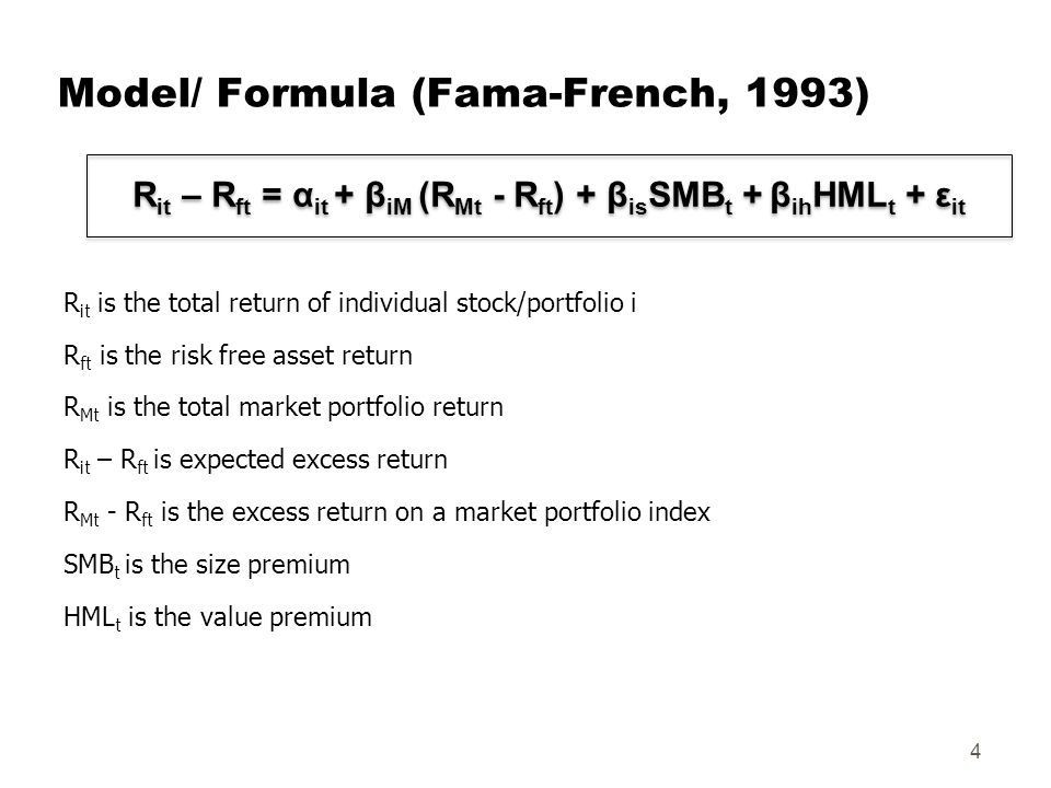
여기서 등장한 alpha 값은 시장보다 잘 나왔을 때, 이를 설명해주는 값으로 CAPM에서 수익 예측시에는 0로 둔다. Fama-French에서도 일단 alpha값은 신경쓰지 말자.

ß가 많아 졌다. 이게 핵심이다. CAPM의 ß만으로는 size effect, value effect가 설명되지 않기 때문에 등장한 ß들이다. Single factor model과 대조되는 three factor model이다. SMB (rSMB)는 small minus big 즉 rSMB,t = rSmall,t - rBig,t 이다. HML (rHML)은 high minus low로 rHML,t = rHigh B/M,t - rLow B/M,t 이다. Small/Big, High/Low value는 어떻게 결정할까? 


fama french model 이미지 검색결과


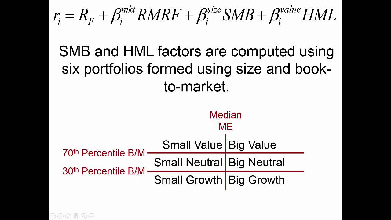
아주 잘 설명된 유튜브 비디오에서 따온 화면이다. Small/Big은 median market value of equity를 기준으로 나눈다. High/Low (즉, Value/Growth)는 Book to market value of equity의 percentile을 기준으로 나눈다. 

며칠 전 블로그에 Warren Buffet의 성공비결을 다룬 글에서 value stock에 대해서 언급했는데, value stock이란 "selling at relatively low prices in relation to their earnings or book value"로, 주로 성숙한 산업군에 있고, 배당금을 많이 준다. 그 반대가 growth stock으로 이해하면 된다.

Fama-French Model은 결국 size와 B/M ratio가 수익을 설명해주고, market ß만이 중요한 변수가 아니라는 것을 말해준다. 하지만 이론적인 모델이 아니며, HML과 SMB가 리스크를 포함하는 개념인지를 명확히 설명해주지는 않는다는 점에서 한계가 있다.

Fama-French Model에서 설명하지 못하는 것이 momentum effect인데, 이는 수익성을 보이던 자산이 계속 수익성을 보인다는 것이지만 근래에 많이 사라졌다고 한다.

그 다음 나오는 마지막 모델이 바로 Arbitrage Pricing Theory (APT)이다. 이름에 Arbitrage가 들어가지만 arbitrage가 없는 상황을 전제로 한다. 

arbitrage pricing theory 이미지 검색결과
*출처: https://www.slideshare.net/mathewrincon/chapter-7-5628056


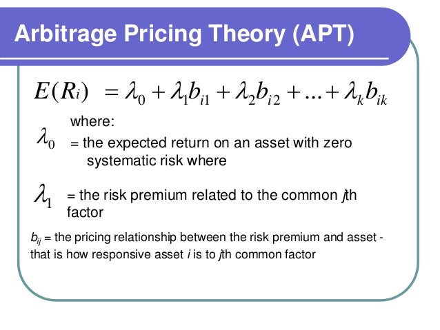
핵심은 위의 수식에서 보듯 여기서는 market premium과 market ß를 사용하는 것이 아니라 거시경제 리스크면 무엇이든 risk factor가 될 수 있다. 인플레이션, 금리 등이다. 그리고 이와 관련된 ß들이 쭉 나온다. CAPM 보다 많은 요인을 고려한 것이다. 

λ는 특정 리스크에 대한 price (premium)이라고 보면 된다. CAPM에서 시장리스크에 대한 price가 E(rm) - rf 였고, Fama-French에서 HML 리스크에 대한 price가 E(rHML) 이었음을 상기해보면 된다.

APT는 CAPM에 비해 assumptions이 많지 않고, CAPM에서 전제로 하는 market portfolio를 가질 필요가 없다. Well-diversified portfolio면 충분하다 (왜 그런지는 잘 이해하지 못했다).

하지만 APT applies only to well diversified portfolios, so idiosyncratic risk might make arbitrage risky. 그리고 APT는 risk factors가 정확히 뭔지 규정하지 않아 조금 애매한 점도 있다.


마지막으로 2013년 The Economist 기사 "The Rise of Smart Beta" 내용을 잠깐 살펴보자. 이는 흔히 passive index fund들이 cap-weighted 방법으로 펀드 내 자산을 구성하는데, smart beta는 조금 더 active 하게 골라서 수익을 더 뛰어나게 하는데 사용되는 베타이다. 여기서는 네 가지 방법을 제시한다.

  1. To give each market constituent equal weight.
  2. Fundamental indexing: to weight each company by its financial characteristics (sales, dividends, assets,or cashflow)
  3. To weight the index in terms of the volatility stocks (with the least volatile being favored)
  4. To use the momentum effect: to buy stocks that have recently risen in price

이 smart beta는 앞서 살펴본 모델들이 여러 가지 factor들을 다 커버하지 못하므로, 대안으로 나오게 된 전략이라고 볼 수 있다. 

이상 투자수익률과 pricing을 결정하는 여러 모델들을 살펴봤다. 이는 향후 투자론의 핵심이 되는 기초지식이니 꼭 이해하도록 하자.


2020년 3월 6일 금요일

MBA Note_Investments_The Secrets of Buffett's Success

Finance 전공과목들을 들으면 역시 Warren Buffett이 종종 등장한다. 지난 Corporate Finance 수업에서는 Warren Buffett과 James Simon을 비교했었다. 그때는 Warren 보다는 Jim의 활약을 다뤘는데, Jim은 Renaissance Technologies 헤지펀드의 설립자이다. Renaissance의 대표펀드인 Medallion fund는 1998년부터 2018년까지 연평균 수익률이 무려 39%에 달한다(after fee 기준). 같은 기간 Warren의 Berkshire Hathaway 수익률이 16%임을 감안하면 대단한 수치가 아닐 수 없다. Jim은 MIT 출신으로 수학을 전공했는데, 여러 가지 회귀분석을 사용하여 투자를 진행했다. 큰 한 방보다는 50% 이상 수익이 예상되는 것에 분산했다고 한다.

뭐, 이건 작년 수업 이야기고, 이번 Investments 수업에서는 역시 Warren의 성공비결을 다뤘다. The Economist Vol. 404, Iss. 8804 (Sep 29, 2012): 77 내용인 The Secretes of Buffett's Success라는 제목의 기사를 바탕으로.

일단 Warren은 항상 콜라를 들고 다닌다. 그만큼 콜라를 사랑하고 콜라의 가치를 보며, 코카콜라의 주주이기도 하다. 즉, growth주보다는 저평가된 value주에 투자를 하는 것으로 유명하다(growth와 value는 Fama French 모델의 HML에서 나오는데, book value와 market cap의 비율이다; book value가 높아야 value주다). 요즘 주식을 투자하면서 코카콜라를 매력적으로 보는 사람들이 얼마나 있을가? 나조차도 주식을 하고 있지만 FAANG이나 반도체, 바이오 같은 요즘 트렌드에 맞는 주에만 관심 있지 코카콜라를 생각해 본 적은 한 번도 없다. Warren은 또한 quality를 투자의 지표로 삼은 것으로도 유명하다(경영진의 quality 등). 즉, 이런 우량주들은 low beta와도 직결된다. 이까진 어느 정도 알고 있던 바다.

Then, what have been the critical factors driving his returns and success? What has been his edge?

여기서 놀랐는데 바로 leverage를 기반으로 투자했다는 점이다. 놀랍게도 Berkshire의 평균 leverage 비율은 60%에 달한다고 한다. 그런데 단순히 돈을 빌려서 투자한 것만으로는 부족하다. Berkshire는 이 돈을 이율 2.2%의 cost of funds로 빌렸다고 한다(1989~2009). 이 기간 동안 미국 Treasury Bill rates 평균은 5%가 넘은 걸 감안하면 정말 싸게 부채를 확보한 것이다!

저렴한 이율로 빌릴 수 있었던 비결은 다음과 같다: Yet the underappreciated elements of Berkshire's leverage are its insurance and reinsurance operations, which provide more than a third of its funding. An insurance company takes in premiums upfront and pays out claims later on; it is, in effect, borrowing from its policyholders. This would be an expensive strategy if the company undercharged for the risks it was taking. But thanks to the profitability of its insurance operations, Berkshire's borrowing costs from this source have averaged 2.2%, more than three percentage points below the average short-term financing cost of the American government over the same period.

아래 그림에서 보면 Berkshire의 투자 alpha 값은 오히려 leverage 없을 때는 마이너스이다. CAL보다 아래에 위치한다(Capital allocation line이지만 실제로는 capital market line, CML이 맞겠다). 그런데 싸게 돈을 빌려서 leverage로 기울기가 가파르게 상승함을 볼 수 있다. Beat the market!


그런데 여기서 주의해야 할 점은 Berkshire의 leverage 후 alpha 값이 플러스가 아니라는 점이다. Alpha 값은 순전히 투자를 allocation을 잘 해서 시장보다 나은 수익률을 말하는 것인데(Alpha, often considered the active return on an investment, gauges the performance of an investment against a market index; 즉, active management return), Berkshire는 그것보다는 비즈니스를 잘 해서 낮은 이율로 돈을 빌릴 수 있다는 점이 저 가파른 기울기를 설명해줄 뿐이다. There's no alpha here!  물론 위에서 설명한 것처럼 우량주를 선택했다는 점이 안정적인 수익을 보장하기는 했지만 말이다.

정리해보면 Warren Buffett의 성공비결은 다음 두 가지이다.

  1. The low-beta nature of the portfolio
  2. Leverage-pretty much

참고로 2020년 3월 현재 Berkshire가 보유한 지분이 높은 업체들은 다음과 같다.

  1. Apple 29.74%
  2. Bank of America 13.46%
  3. Coka Cola 9.15%
  4. American Express 7.8%
  5. Wells Fargo 7.18%

지금 코로나19 발로 미국 증시에 본격적인 조정세가 오고 있다. 물론 민주당 경선에서 샌더스의 약진, 그리고 10년주기 불황설의 대두 등으로 연준이 0.5% 금리를 인하했음에도 불구 장은 하락 중이다(내 주식 ㅠㅠ). 지난 2월 24일 Warren Buffett이 CNBC에 나와서 인터뷰를 했는데, 이 조정은 곧 지나갈 것이며 지금 Apple을 담기에 가장 좋은 시점이라고 말하기도 했었다(Apple picking 이네 ㅋㅋ). Berkshire가 30%나 보유한 회사기 때문에 약간의 의도가 섞여 있다고 보지 않을 수 없지만, 나 역시 곧 지나갈 시련이라 생각했었다. 그런데 약 2주가 다 되어 가는 지금, 미국 증시는 점점 떨어져만 간다. 이번 1분기 이후가 관건이겠다. 

2020년 2월 24일 월요일

MBA Note_자사주 매입 (Buybacks)

Bio Pub인데 요즘 너무 MBA 노트가 된 것 같아 바이올로지에게 미안하다. 잠깐만 외도할게.

이번 Investments 수업의 class 5에서는 equity에 대해 다룬다. 여기서 자사주매입도 나오는데, 이는 지난 Corporate Finance 수업 때도 다뤘던 내용이라 복습겸 블로그에 남겨본다.

먼저 다룬 페이퍼는 Ryan, Vincent. “Rethinking Buybacks.” CFO Magazine, July 2014, pp. 21-24. 였다. Buyback, 혹은 repurchasing their company's stock으로 표현되는 자사주매입은 회사에 캐시가 많을 때 고민할 수 있는 전략이다. 2008년 금융위기 이후 회사들은 캐시 보유량을 늘려 나갔고, 이 남아도는 캐시를 어디에 투자할지 고민한다. 이때 생각할 수 있는 방안은 흔히 다음과 같다.


  1. 사업에 재투자 (to organic growth)
  2. 주주 배당 지금
  3. 자사주매입

나 같이 R&D로부터의 혁신을 꿈꾸는 사람에게는 1번이 가장 매력적으로 보이지만, 페이퍼에서는 1번의 경우 이미 시장은 포화됐고 재투자의 리스크 대비 수익이 확실히 보장되지 않는다고 언급한다. 2번의 경우 주주가치 실현이라는 목표가 회사에 있을 경우 좋은 방법이긴 하지만 문제는 배당금은 세금을 물기 때문에 그리 매력적이지는 않다고 한다. 그래서 남은 것이 3번인데, 자사주매입의 장점은 다음과 같다.

  1. EPS 증가: 자사주매입하면 주식수가 줄어드므로 당연히 주당이익은 늘어난다. 이를 통해 주주들은 주식을 팔아서 capital gain을 얻을 수 있다. 물론 미국에서는 모든 주식매매 이익에 대해 세금을 물지만, 이는 배당금과 달리 주주의 의지대로 원하는 시점에 이익을 챙기고 세금을 물 수 있는 선택권을 준다.

  2. 적대적 인수로부터 보호: 우리 회사를 먹으려는 상대방으로 하여금 먹을 주식이 없게 만들어 버린다. 이것도 상당히 많이 사용되는 전략이다.

  3. 저평가 우량주라는 신호: 회사가 본인의 가치를 알기 때문에 싼 값에 매수하려고 한다는 기대가 시장에 퍼져나갈 수 있다. 보통 1번과 함께 자사주매입 발표후 주가가 오르는 원인이다.

  4. 경영진 보상: 경영성과가 좋을 경우 자사주로 보상할 수 있는데 이의 소스가 된다.

  5. D/E 유지: Debt대비 equity의 비율이 오르기 좋은 환경에서 자사주매입을 통해 equity의 비중을 줄인다. Balance sheet에서 treasury stock(자사주)은 stockholder's equity 항목에서 차감된다. 

  6. 법인세 유리: 이건 아래 Investments 수업에서 다룬 내용이다. 보통 자사주매입을 위해 부채로 돈을 빌리는 경우가 많은데, 이럴 경우 tax shield 효과를 볼 수 있다 ("Since interest paid on debt is tax-deductible, whereas interest earned on cash is taxable, by increasing its net debt to finance buybacks or dividends, a firm cuts its tax bill.") 하지만 부채가 늘어나는 것은 risk도 수반한다는 것은 언제나 염두에 둬야 한다.

그 다음 다룬 페이퍼는 Michel, Allen (Corporate Finance 교수님이다), Jacob Oded, Israel Shaked. “Not All Buybacks are Created Equal: The Case of Accelerated Stock Repurchases.” Financial Analysts Journal, Vol.66, No. 6, 2010, pp. 55-71. 인데 간단하게만 다뤘다. 

여기서 등장하는 개념은 ASR (accelerated stock repurchase)인데, 보통 자사주매입의 형태인 OMR (open-market repurchase)와 대조되는 개념이다. 위에서 다룬 장점들은 OMR 기반이라고 보면 된다. ASR은 아주 신속하게 자사주를 매입하는 형태인데, 이 페이퍼에서는  ASR 이후에는 주가의 행보가 OMR처럼 양호하지 않았다는 것을 보여준다. 투자자들도 ASR을 좋은 뉴스라고 보지 않는다. EPS에도 큰 영향이 없다고 하는데 이유는 EPS 산출시 사용되는 주식의 수는 당기당 평균 주식수로 계산하기에 그 효과가 희석되기 때문이다. 더군다다 ASR은 내부정보 활용하면 무조건 insider trading이므로 경영진들은 주의해야 한다. 예컨대 월마트에서 매출 오를 것 알고 ASR을 진행한다고 하면 내부거래이다.

자, 여기까지가 지난 가을학기 Corporate Finance에서 다뤘던 자사주매입의 내용이다. 내일 Investments 수업에서 다룰 내용은 어떻게 다를까?

내일 수업에서는 The repurchase revolution; Share buy-backs, The Economist; London Vol. 412, Iss. 8904,  (Sep 13, 2014): 71-73.를 다룬다. 얼핏봤는데 더 심오하다(일단 필자가 너무 어려운 단어를 좋아한다 ㅜㅜ). 수업 후 후기를 남겨보겠다.

(후기) 이 페이퍼는 자사주매입에 대한 비판적인 시각이 깔려있다. 교수님께서 이 페이퍼에서 가장 주목해야 할 자사주매입의 단점으로는 회사가 자사주를 buy high, sell low 할 수 있다는 점이다. 단기적으로 주가는 오르지만, 결국 회사가 다시 파는 시점은 당장 현금이 필요한 때, 즉 회사 상황이 좋지 않을 때일 확률이 높기 때문이다(제대로 이해한 것 맞나?). 

(후기) 이후 Problem Set 3에서 자사주매입 문제가 나와서 여기 옮겨본다:

5. An article in the financial press identified the following six opinions and/or  assertions related to share buybacks: 
(i) A company buying back itself is “unnatural”. 
(ii) Buybacks create unequal shareholder wealth (i.e., winners and losers) 
(iii) Companies’ main motivation for buybacks is to manipulate either their stock  prices or their earnings per share.  
(iv) Firms should reinvest the money back into themselves instead. 
(v) Buybacks lead to low rates of investment by such firms. 
(vi) If buybacks rise after a change in the corporate tax code, then the change  was not in the public interest. 

Pick two of these statements and briefly discuss a counter-argument to each of  them. Also state whether you mostly agree or disagree with each of the two  statements you choose to address. 

나의 답 (reinvest에 대해서는 소신 발언 했는데 점수 깎이진 않은 것 같다):
(iii) Counter-argument: The main motivation for buybacks would be protection of ownership from hostile acquisitions or securing shares for management rewards. 

I agree that a company’s stock prices or EPS would increase after their announcement of buybacks since it could a signal that the company’s stock is undervalued and/or the number of shares outstanding will fall so that EPS will grow. But if they do not perish the treasury stocks they bought back, then the number of stocks would not change. Actually many Korean companies do not eliminate treasury stocks they repurchase. 

(iv) Counter-argument: Reinvesting into a firm won’t provide enough return for the risk. 

Financially, investing in organic growth would not look attractive in terms of increasing value of a firm in a short period of time, but the leading businesses these days are actually based on innovation in technologies/sciences and manufacturing, so I believe reinvesting is the way increasing true value of a firm for the long shot. This will increase the fundamental value of a firm with solid streams of cash flows in the future.

정답:
These statements all come from an opinion piece (Schumpeter) in The Economist.  All of these arguments are actually called “muddles” by the author of this article.  Here are the counterarguments the author poses: 

(i) Buybacks are like dividends as cash moves from the firm to its owners. The advantage here is flexibility; unlike dividends, shareholders can elect whether or not  to participate, and firms can start and stop buybacks without disappointing investors  to as great an extent as would be the case if they lowered their dividends. 

(ii) One analogy might be thinking withdrawing money from an ATM makes you richer (it does not). Buybacks can transfer wealth between shareholders because if  you sell at a price that turns out to be low, the other shareholders will benefit, but their gains could just as well result in greater shareholder equality (i.e., those who held on started out less well off than average) as in greater inequality. 

(iii) This claim is hard to justify or confirm because buybacks are small relative to the  value of the overall market, representing just 2% of the total, and only 1% for firms in  the S&P 500. In addition, rules prevent firms from dominating the trading in their  own shares on any given day. It is true if executive pay plans are poorly designed  around earnings per share they can artificially encourage buybacks, but of the 20  largest repurchasers in mid-2018, three-quarters did not have EPS as a main element  of their pay plans 

(iv) Buybacks are dominated by firms that specialize in intellectual property, and they  are unable to reinvest all of their profits at acceptable rates of return. For example,  had Apple reinvested all of the money it had used to repurchase stock over the past  decade, its physical plant would be six times larger than is currently the case. A  healthy company is one in which abnormally high profits are recycled by the financial  system, not one in which fat incumbents get ever larger purely for the sake of size.  

(v) A 2017 study by Federal Reserve economists found little evidence that buybacks  lead to low rates of investment. As firms’ cash flows have risen relative to GDP since  the 1990s, a lower proportion has been spent on investment, which is a case of the  denominator rising, rather than the numerator shrinking. Investment remains in line with 1990s’ levels. Surges in buybacks and investment can actually be  complimentary, rather than serve a substitutes for each other: during Q1 2018, 64% of  firms that boosted buybacks also boosted investment. In fact, these firms were slightly  more likely to boost investment than were the nonbuyback firms. 

(vi) This statement is not accurate. Better measures would be a) whether overall  investment rises b more than the amount of the tax break, which appeared to be a  possible outcome in 2018, b) whether firms’ wage bills are rising, and c) whether  these effects will last. 

Source: The Economist. (2018, June 2). Six muddles about buybacks. 

Personally, I agree with all of these counterarguments, although I do believe some  managers use buybacks to boost performance measures tied to their compensation  plans. As for the “public interest” argument, it is also worth noting the most recent  change in the U.S. tax law allowed companies to repatriate hundreds of billions of  dollars back to the United States after paying incremental taxes at favorable rates.  While this additional revenue to the U.S. Government was not a huge windfall, one  can argue this change in the law did serve to make the flow of capital more efficient,  which may ultimately be in the public interest. 


2020년 2월 22일 토요일

Smaht Pahk

페이스북 2020.2.3. 게시글

"Smaht Pahk"

지난주 회사 동료가 동영상 하나를 보내왔다. 수퍼볼 때 방영되는 광고 중 하나라는데 현대였다. 미식축구 룰도 제대로 모르는, 그리고 아직 미국문화 새내기인 나는 그냥 현대차가 열심히 했네 정도로 보지도 않고 넘어갔는데, 회사의 미국, 특히 보스턴 토박이 친구들이 자꾸 광고를 따라하며 웃었다. 광고에서 보스턴 특유의 억양이 잘 표현됐다는 것이다(보스턴은 처음 영국인들이 정착한 곳이라 그런지 약간 영국영어인듯 아닌듯한 억양이 섞여있다). 알아 듣기에도 급급한 나인지라 억양까지 눈치 챌 여유는 없었지만 동료들이 말해주니 그런가 싶었다.

그런데 잘 보니 출연진들이 대단하다. 캡틴아메리카 Chris Evans와 미드 오피스의 주연 John Burke Krasinski다. 모두 매사추세츠 출신이라고 한다. 이야 현대 돈 좀 썼네라는 생각.

방금 The Boston Globe에서 보내는 Talking Points PM이라는 이메일 뉴스에 이에 대한 내용이 실렸다. 적어도 보스턴, 매사추세츠에서는 어느 정도 바이럴한가 보다.

실린 내용은 이렇다. 이 광고의 감독인 Bryan Buckley는 지금까지 60편 이상의 수퍼볼 광고를 찍었다고 한다. 하지만 이번 현대차 광고에 대한 애정이 느껴지는 대목: Bryan Buckley has directed more than 60 Super Bowl ads. It's hard to pick favorites. But he admits it will be tough to top the experience of shooting this one. 제작 뒷이야기를 들여다 보니, 현대의 인하우스 에이전시인 Innocean이 Buckley 감독의 프로덕션사 Hungry Man에 연락했다고 한다. 이미 대본과 출연진 확보는 마친 상태였다고. 감독 또한 예전에 보스턴 지역에 살았기에 거절할 수가 없는 조건들로 반찬은 꾸려졌다. 또 현대는 현장감을 살리기 위해 촬영 때 배우들이 보스턴으로 건너오도록 경비를 다 대줬다고 하고, Buckley 감독은 이를 칭찬했다. 현대가 잘 했네.

Bloomberg에 따르면 올해 수퍼볼 광고를 내보내려면 30초에 $5.1에서 5.3M, 즉 60억원을 웃도는 비용을 내야한다고 한다. 현대광고는 1분짜리니 방송에만 120억원 이상을 지불했겠구나. 하지만 이번에는 왠지 마케팅덕을 좀 볼 것 같다.

현대의 마케팅 하면 생각나는 게 있는데, 작년 마케팅 수업 첫 시간에 현대차 사례가 소개된 적이 있었다. 2008년 금융위기 때 미국에서 자동차 수요가 36% 급감했고, 대부분의 업체들은 할인전략을 펼치고 있을 당시. 현대는 조금 다르게 접근했는데 소비가 줄어든 이유가 뭔지에 대한 근본적인 질문을 했고, 알아낸 바로는 소비심리 위축의 배후에는 실직 리스크에 대한 두려움이 있었다고 한다. 그래서 선택한 마케팅 전략은 구매 후 1년 이내에 직장을 잃거나 감봉될 경우 신용에 지장 없이 환불해주기. 이름하여 Hyundai Assurance. 이 프로그램은 2009년 1월에 도입됐고, 업계는 1963년 이래로 1월 판매 최대 급락(37%)를 겪었는데, 현대는 당월 매출이 두 배로 뛰었다고 한다. 와우!

아무튼 타지에서 가끔 이런 일이 있으면 웃을 수 있어 좋다. 보스턴에 현대차 주재원분도 계신데 ㅋㅋ 으쓱하시겠네.

근데 보스턴에서 smaht pahk? 서울가보세요

파괴적 혁신?

페이스북 2019.11.23. 게시글

파괴적 혁신?

내가 종사하는 분야에서 disruptive innovation이라는 용어가 들리기 시작한 것은 기억으로는 '15년, '16년 정도로 거슬러 올라간다. 한참 미국의 바이오 스타트업들이 주가를 올리고 있을 때였고(pharma, non-pharma 아울러), 테크 쪽에서도 우버나 에어비앤비가 산업의 지각을 흔들고 있을 때였다. 그리고 곧 한국 매체들에서도 이 표현이 자주 등장하기 시작했다.

그런데 이상한 점이 있었다. 한국이든 미국이든 disruptive /디스럽티브/를 /디스트럽 or 디스트럭티브/로 말하는 사람들이 적잖이 보였던 것이다. Disruptive? Distruptive?(뭐지 이 족보 없는) Destructive? 그리고 한국 매체에서는 이를 "파괴적 혁신"으로 번역하였다.

Google 사전에 disruptive를 검색해보았다.
causing or tending to cause disruption

뭐야 이거, 순환정의의 오류잖아. 다시 disruption을 검색해봤다.
disturbance or problems which interrupt an event, activity, or process

뭐 광의적으로 유사한 선상에 있지만 그래도 파괴라는 단어와는 조금 거리가 있는 듯하다. 한글로 정의를 찾아봐도 "지장을 주는" 정도이다. 한국에서 파괴적이라는 형용사를 차용한 것을 보면, 아마 언어불문 destructive와 혼동하여 사용되고 있는 경우가 적지 않음을 시사하는 것이 아닐까.

정의에 집착하자는 건 아니지만 원래 이 표현이 의도하는 바와 다르게 해석될 수 있기 때문에 한번 짚어볼 필요는 있겠다.

Disruptive innovation은 Harvard Business School의 Clayton Christensen 교수가 1995년에 처음 도입한 말이다. 요는 다음과 같다. 대기업은 보통 현재 주요고객의 눈높이에 맞춰 제품의 성능을 개선시키는 sustaining innovation을 추구한다. 이 주요고객들이 이런 개선에 대해 반응도 좋고 지갑도 잘 열기 때문이다. 그런데 이경우, 제품은 어느 순간 스펙이 "너무" 좋아져버리게 된다. 물론 가격상승도 뒤따른다. 세상에는 적당한 기능에 적당한 가격을 바라는 소비집단도 있다. Disruptive innovation은 바로 이런 집단을 타겟으로 한다. 처음에는 저렴하고 높지 않은 스펙으로 소수고객들에게만 어필한다. 이때 로우스펙이지만 뭔가 차별화된 기술이 있다. 대기업은 이들을 신경쓰지 않는다. 그들의 기준에 별 볼일 없는 제품이다. 하지만 언더그라운드에서는 언더독들이 이런 소수고객들에게 어필하기 위해 그들만의 리그가 펼쳐지고 나름의 sustaining innovation 지하버전이 진행된다. 여기서 살아남는 제품은 어느 순간 괴물이 되어 있고, 일반고객들도 눈을 돌리기 시작하며, 결국 대기업들은 이들에게 주요고객마저 빼앗긴다. 따라가기엔 때가 이미 늦었다. 이렇게 아래서부터 "야금야금" 시장을 잠식해 나가는 것이 바로 disruption의 핵심이다. 확실히 파괴와는 거리가 조금 있어 보인다.

Christensen 교수는 본 개념에 대해 2015년 다시 입을 열었다. 이 표현이 등장한지 20년 만이고, 처음 소개했던 Harvard Business Review에 다시 글을 실었다. 오용. 제대로 의미를 파악하지도 않고 자신들이 하려는 일을 옹호하기 위해 어설프게 사용하는 사례를 너무 많이 목격했다고 한다. 그리고 이론에 대한 추가설명이 이어진다. 여기선 스킵하고.

자, 이미 그렇게 되었으니 파괴적 혁신이라고 번역하는 것은 큰 문제가 아니겠다(증강현실도 현실연장이라고 번역했으면 훨씬 쉬웠을 걸 뭐 이미 그렇게 번역되고도 잘 쓰이고 있으니 ㅋㅋ). 그래도 적어도 이 표현에서는 파괴적이 급진적, 폭발적을 일컫는 것이 아님은 염두에 두고 있어야겠다.

그리고 자, 위의 정의에 맞춰 본다면 우버는 파괴적 혁신의 사례가 아니다(지금 기업가치와는 별개로, 우버가 아주 잘 나갈 때 우리가 이 업체를 바라보던 감정으로 이 문장을 바라보자).

주변에서도 이 표현을 혼동해서 쓰는 분들이 많은 것 같아 그냥 그런가보다 하고 있었는데, 마침 한 수업에서 이 개념을 다시 만나게 되어 반가웠고 나도 재차 확인할 수 있는 계기가 되었다.

무엇보다 보스턴에 와서 지내다 보니 HBS에서 Christensen 교수님 아래에서 일을 했던 분도 친구가 되었다(친구 맞죠?). 공자 앞에서 문자 읊었는데 그분이 이 글에 혹시나 있을 잘못된 내용을 지적해 주신다면 크나큰 영광이겠다 ㅎㅎ
[선별 댓글] Christensen 교수 제자이자 KSV벤처캐피탈 대표 Spencer님의 댓글
Spencer Nam 크리스텐슨 교수의 흥미로운 관점중의 하나는 “세상에는 두가지 종류의 고객이 존재하는데 (1) 현재 제품을 구매하려는 고객과 (2) 현재 제품과 비슷한 성능의 제품이 필요한 고객이 있다”는 것인데 보편적으로 시장과 기업은 (1)만 보고 (2)을 무시하거나 아니면 가격 문제로 문제의 근본을 축소시키다 보니 결국 구매를 하는 고객이 줄어들면 가격을 높여서 구매하는 고객들에게서 더 쥐어짜려 하다보니 (2)을 타겟하는 회사들이 결국 (1)을 타겟하는 회사들을 잡아먹게 된다는 것이죠.

Charles Schwab와 Robinhood

페이스북 2019.10.8. 게시글

인더스트리 판도가 바뀌고 있다. 사업모델도 너무 다양해지고 그래서 기존 시각으로 보면 이해가 되지 않는 것들이 아주 많이 생기고 있다.

아래 기사는 최근 발표한 미국 최대 온라인 증권사 찰스슈왑Charles Schwab에 대한 이야기다. 주식거래수수료 등 모든 수수료를 폐지하겠다는 다소 충격적인 발표. 왜?

몇 년 전 미국에 나왔을 때 로빈후드Robinhood라는 앱 광고를 보고 뭐 이런게 다 있지 했던 기억이 난다. 주식거래 앱인데 수수료가 없다는 거다. 도대체 이 회사의 사업모델은 뭐야? 지인찬스를 통해 고객계좌 잔금 이자수익, 프리미엄계정 가입 수익(소위 freemium이라 불리는) 등임을 알게 됐다. 좀 더 찾아보다 "payment for order flow"라는 모델도 알게 됐는데, 고객이 신청한 거래를 제3자(Citadel Securities나 Virtu Financial과 같은 온라인거래사)에게 위임하고, 이 라우팅의 대가로 로빈후드는 돈을 받는다. 한 마디로 브로커 역할이다. 이런 모델들로 로빈후드는 수수료 안받고 매출을 낸다.

대형 증권사는 이런 의적들에게 고객을 뺐기고 있다. 임꺽정, 장길산까지 나올 기세. 그러니 슈왑도 이런 다소 극단적인 조치를 취한 것이다. 수익이 낮은 수익모델에 기댈 수 밖에 없는 판이 이미 짜여졌다. 고객은 만쉐이. 증권사의 직원들은 비용절감 나아가 구조조정 압박에 한 동안 시달릴 생각하니 불쌍하지만.

이런게 가능한 이유? 세 가지가 떠오른다. 테크의 발전. 플랫폼 전성시대. 무엇보다 미국의 남아도는 캐쉬. 뭐, 곧 불황이 온다는 이야기도 많지만. 쩐이 많으면 아이디어 기반 테크 스타트업에 많은 플로우가 생기고, 걔 중 살아남는 녀석들의 여파는 어마어마 하다. 그래서 수수료로 돈도 못 버는 로빈후드의 기업가치는 자그마치 $8 billion, 지금 환율로 거의 10조원에 육박한다. 물론 최근 소프트뱅크SoftBank-위워크WeWork 여파로 기업가치나 시가총액에 대한 비판적인 시각은 많지만, 설령 로빈후드가 망한다고 해도 이미 공짜를 맛본 고객들을 대상으로 슈왑이 쉽사리 다시 수수료를 매기지는 못할 거다. 말인즉 테크가 곳곳에 스물스물 스며든 플랫폼 사업이 당분간 세상을 변혁시켜 갈 것이라는 점은 자명하지요.

요즘 미국 스타트업의 사업모델은 기괴한 것이 많다. 내가 일하는 산업바이오 분야도 마찬가지다. 요즘 이 분야마저 투자 잘 받는 친구들의 사업모델은, 단순 제조/서비스업 이상의 무엇이 있다. 어떤 바이오업체는 스타트업 주제(?)에 자꾸 자회사를 만들어 그 회사들의 지분가치 올리는데 집중하는 금융투자업을 모델로 삼는다. 물론 돈놀이에도 스토리텔링은 필수. 제조업의 시각에서 보면 crook. 돈 끌어오는 시각으로 보면 천재. 이 케이스에서는 난 아직 제조꼰대 마인드가 좀 있지만.

여튼 시사점. 정신 바짝 차려라.

* 페이스북 링크: https://www.facebook.com/illozika/posts/10158828098115278

글로벌 단국적 기업?

페이스북 2018.8.14. 게시글

글로벌 단국적 기업?

보스턴에 나온지도 이제 두 달이면 이 년이다. 그 동안 작은 오피스를 운영 아닌 운영 해오면서 마주했던 몇 가지 일들 더하기 이곳 스타트업에서 일하는 한국인, 현지인, 이곳 다국적대기업에서 일하는 한국인, 현지인들을 만나다 보면 "corporate culture"에 대해서 많이 생각하게 된다.

현지직원들과 본사를 연결시켜주는 것은 전체의 비전과 미션을 동기화 시키는 측면에서 매우 중요하다. 대부분의 경우는, 결국 사람 일인지라 사람으로 해결이 되지만, 간혹 쉽지만은 않은 일들이 발생하곤 한다.

Corporate culture, 조직문화. 앞서 내가 겪은 사람들을 크게 두 가지 축으로 분류해봤다. 스타트업 vs. 대기업, 그리고 한국 vs. 현지. 간단히 총 네 가지의 기업체질이 나눠진다. 여기서 간혹 이슈를 혼동하는 소위 "orthogonal issue"가 발생하기도 한다. 즉, 대기업으로서 가져야 하는 조직문화의 당위성을 한국기업이니까로 치부해버리는 경우가 종종 있다. 이런 오해들을 풀어주기 위해서는 매니져가 소통을 잘 해야 한다. 잘 하는 건 딴 게 없다. 자주하면 된다.

그런데 저런 종류의 혼동이 아닌 진짜 한국기업이 지니는 이슈들도 있다. 이건 비단 한국기업만의 문제는 아니고 일본, 중국 등 동북아의 기업문화가 유사할 것이다. 도요타나 혼다가 미국에 발을 들여 놓았을 때 겪었던 많은 충돌들이 그것일테다 (이를 다룬 영화도 있었는데 뭐더라?).

처음 여기 다국적회사에 일하는 연구원들 (연구원이다. 법무, 재무 등은 한국보다 더 빡세게 일하시더라)을 보며 조금 놀랐다. 출퇴근에 대해 물으면 "어, 뭐 딱히 그런 건 없는데 보통 9시쯤 가서 5시쯤 나오나?" 대략 이런 반응이었다. 물론 학위 때 취리히에 잠깐 나갈 기회가 있어 다섯시면 온 학교에 불이 꺼지는 것을 직접 목격하고 적잖은 충격을 먹기도 했었으나, 미국의 글로벌 탑 기업-영리기관-의 연구소들도?

하루는 현지 친구가 재밌는 기사를 봤다며 말을 걸어왔다. OECD 국가들의 노동생산성이었다. 한국은 노동시간으로는 최상위급, 생산성으로는 최하위급이었다는 것이다. 자, 내가 너에게 무슨 말을 해주리. 솔까 한국애들이 니들보다 훨 똑똑해. 여기와서 살아보니 확실히 알겠어. 근데 객관적인 지표가 없다. 여기서 한국인의 똑똑함과 생산성을 강조해봤자 그들의 눈에는 파시즘과 크게 달라 보일까. 말을 아낀다.

한국의 조직문화로 비롯된 쓸데 없는 노동시간만이 이를 설명해준다. 아까 스위스에 갔었다고 했다. 이 학교에서 나오는 논문들 양이나 질을 보며 투여시간과 생산성 공식에 대해 진지하게 생각해볼 수 있는 계기가 되었다. 한국인의 똑똑하다고 믿는 나로서는 능력을 시스템이 저해하고 있다는 결론으로 치닫는다.
그전에, 우리가 생각하는 똑똑함의 기준이 잘못되었나?

그것도 일부 말이 될 수 있다. 우리는 손이 좋고 머리회전이 빠르지만 가끔 거기에만 너무 빠져드는 경향이 있다. 거시적인 시야를 똑똑함이라고 정의한다면, 그 부분을 우리는 간과하고 있다고 할 수도 있겠다.

그게 아니라 정말 똑똑한 게 똑똑한 것이 맞다면, 잘못된 방향으로 인해 똑똑함이 "translation" 되지 않은 것일 수도 있다. 똑똑한 사람들을 제대로 이끌어주는 리더의 부재. 매출이나 시총으로 볼 때 미국의 선도기업은 애플, 아마존, 구글, 페북, 마이크로소프트일테다. 이들을 설립한 사람은 문과냐 이과냐. 하이텍뿐 아니라 바이오 분야의 다국적 업체들을 봐도 대부분 과학자들이 세웠고 이들이 리드한다. 혁신의 인사이트는 직원보다 더 전문가인 리더로부터 나온다. 그런데 한국은?

(적어도 기술업체에서) 리더가 과학, 기술적 비전을 제시할 수 없다면 결국 관리 운영으로 승부를 보려고 하고, 거기서 나오는 것이 관료적 시스템이다.

물론 한국 스타일로 세계를 씹어 먹고 있는 몇몇 기업들이 있다. 서구가 세상을 지배한 게 불과 얼마전이냐. 다시금 아시아로 패권이 넘어올 수도 있겠으나, 어쨌든 현 시점만 놓고 보면, 적어도 글로벌에서 정말 글로벌스러운 사업을 하고 싶다면, 위에서 언급한 내용들에 대해 진지하게 생각해봐야 할테다.

그렇게 외국에만 나오면 내성적인 일본인들. 그런데 Takeda가 세계적인 제약사로 어떻게 성장하였는지. 글로벌 다국적 기업으로 성장하려면 단국적적인 문화를 어떻게 극복할지 깊이 생각해봐야 하겠다. 그게 아니라면 적어도 한국 조직문화의 당위성을 설명할 수 있는 무언가는 있어야 하겠다.

애국심으로만 현지친구들과 논쟁하기에는, 아직 무언가가 필요하다.

* 페이스북 링크: https://www.facebook.com/illozika/posts/10157587045195278

[선별 댓글] Boston University 경영학부 김종성 교수님 댓글

Jay S. Kim 이를 다룬 영화? Gung Ho, 1986년 개봉된 영화. 일본 자동차 회사가 "망해가는" 미국회사의 공장을 인수한후 생기는 여러가지 culture crash 와 integration 을 다룬 코메디. Michael Keaton 주역. 90년대 한국기업의 글로벌진출을 준비하면서 대기업 임직원에게 보여주기도 했던 classic. 시사점과 해결책을 찾게 도와줍니다.

Jay S. Kim Joon Jin 진준영박사님이 중요한 문제를 제기해 주셨습니다. 한국기업(사람)이 미국(다른나라도 마찬가지)에 진출하면 바로 와닿는 의문입니다. 해결하지 않으면 사업목표와 전략에도 심각한 영향을 미치는 근본적 문제. 이곳 보스턴에서 활약하는 한인, 교포, 함께 토론해 보아야겠습니다. 또하나의 포럼을 만들어야겠어요.

2020년 1월 26일 일요일

MBA Note_Investments_Class 1: Asset and Security Classes, Investment Companies and Mutual Funds

Finance concentration을 위한 다른 수업, investments를 이번 봄 학기에 듣는다. 최근 미국 주식에 관심이 많이 생겨서 재미있게 들을 수 있을 거라 기대 중이다. 그런데 용어들이 벌써 어렵다. 그리고 내 머리는 자연과학이나 인문학은 그럭저럭 따라가는 편인데, 사회과학에는 조금 약한 것 같아 살짝 걱정도 된다. 그래도 한 한기 지나면 뭔가 남을 거라 믿는다.

이번 수업의 lecturer는 James Welch라는 분이다. Harvard College를 나오셨고, 월가에서 JP Morgan 등에서 꽤나 굵직한 경력이 많으신 분이다. 왠지 월가의 이미지는 딱딱하고 냉철한 사람들로 가득할 것 같고, 그래서 영어도 빠를 것 같았는데 전혀 그렇지 않고 배려심이 많아 보여 한 시름 놓았다.

처음 다룬 개념은 투자(investing) vs. 저축(saving). 아껴두냐 리스크를 감안하고 부풀릴 것이냐가 핵심이다. 수업 후 이메일로 질문한 아래 내용이면 충분히 설명될 것 같다.

Q. As to the concept we learned, I got a point that saving is just keeping our assets without taking risks. To that point, are saving in bank and investing in T-bill so different? (They look so similar in terms of earning stream, i.e. interest vs. coupon and low risks in both, except that fact that we could get a bond with a discounted price).

A. If you consider investing in very safe assets (i.e., T-Bills and/or bank deposits) to be "saving", then there is really a continuum between savings and investing. However, for the purposes of last Tuesday's discussion, I wanted people to understand that setting money aside is the "saving" part, while putting it to work to earn more money is the "investing" part.

투자시 고려해야 할 사항이 몇 있는데, 유동성(liquidity), 투자시계(investment horizon: planned liquidation date), 세금 등이 있고, 또 labor income risk를 hedge하기 위한 니즈도 있다고 한다. 마지막 요소는 선뜻 이해가 가진 않는다. Labor income risk? 구글링을 조금 해보니 보통 시장 상황에 따라 labor income도 volatility, 즉 리스크가 변하고 이를 헷징하기 위한 여러 투자가 진행된다고 한다. 혹은 월급 리스크가 정도가 서로 다른 직장으로 이직할 때 이를 헷징하기 위한 투자전략도 바뀐다고 한다. 보통 대기업에서는 월급을 리스크로 보지는 않는 것 같은데, 그래서 잘 이해는 안가지만 그런 개념인가 한다. 아무튼 이를 위해 분산투자 전략을 세우는데, income 일부를 직장회사에 재투자(주식을 산다거나) 하는 것은 헷징이 아니라 오히려 집중화 시키는 결과를 초래한다고 한다. 회사의 리스크는 월급이든 지분(자본)이든 동일 할 것이니 맞는 말이다.

유가증권(securities)은 "individual claims on specific assets"으로 정의한다. 잘 정의한 것 같다.

투자프로세스는 1) Asset Allocation, 2) Security Selection으로 이뤄진다. 1)은 단기금융시장(money market), 고정수익유가증권(보통 채권), 주식, 부동산 등 중에서 어디에 투자할지 고르는 과정으로, 일반 투자수익의 75%은 이 배분전략으로 설명이 가능하다고 한다. 패시브투자의 경우 100% 설명이 가능하다고 하니, 그 만큼 중요한 스텝이다. 2)는 한 단계 더 나아가 예컨대 주식이면 어떤 종목을 살 것인지 고르는 과정이다.

위에서 패시브투자라는 용어가 나왔는데, 투자는 액티브투자와 패시브투자로 나눠볼 수도 있다. 패시브는 인덱스투자를 생각하면 쉬운데, 전체 시장을 반영할 만한 다양성으로 투자를 하고 그냥 놔두는 수동적인 방법이다. 전체 시장의 평균수익 정도를 노리면서 대신 비용은 적게 드는 방법이다. 반면 액티브투자는 평균보다 높은 수익을 노린다. 이것저것 조사해서 종목을 고르는 것으로, 시간과 비용이 상대적으로 많이 든다. 비용은 트레이딩 비용도 있고, 또 보통 전문가에게 위임하는 경우가 많으므로 여기도 비용이 든다.

Asset은 real asset과 financial asset으로 나뉜다. 말이야 쉬운데 예를 들면 특허는 둘 중 어디에 속할까? 답은 이따가. Real은 실제 재화나 서비스를 생산하는데 사용되는 자산, 공장, 설비, 인적자본 등을 일컫는다. 일반 가구(household)의 real assets을 보면 대부분 부동산이고, 그 다음이 가전제품과 같은 consumer durable이다. 반면 finance asset은 "claims on real assets or claims on asset income"으로 정의한다. 이는 예금이나 보험, 연금, 주식, 펀드 등으로 이뤄진다. 재밌는 것은 financial asset은 무조건 누군가의 채무와 상계된다는 점이다. 그래서 경제의 "net wealth"를 구해보면 오롯이 real asset만 남게된다. Real asset의 궁극적인 오너는 가구, 비영리단체, 정부이다(기업은 없다, 왜 없지?). 특허는 real asset이다(경제학에서는 특허를 "good"으로 분류한다. Good과 service의 차이는 재판매 가능한지, 즉 property right의 유무에 따른다).

대부분 투자는 개인보다는 investment firm을 통해 진행되는데, 이를 통하면, 1) instant diversification, 2) 전문성(및 리서치 비용 감소, 저평가 증권 잘 찾아주고), 3) 거래비용 감소, 4) 관리가 잘된다고 한다. 규모의 경제가 적용되는데 리서치도 많은 고객의 자산을 대상으로 하다보니 고객 간 분배가 되므로 저렴해지고, 대규모 거래를 하면 수수료도 떨어지니깐 설명이 된다.

뮤추얼펀드. 인터넷 정의를 빌리자면 "회사형 투자 신탁 가운데 개방형 펀드. 증권 투자자들이 주식을 매입해 주주로서 참여하는 한편 원할 때는 언제든지 주식의 추가 발행, 환매가 가능한 투자 신탁으로, 미국 투자 신탁의 주류를 이룬다."고 한다. 혹은 "뮤추얼펀드는 유가증권 투자를 목적으로 설립된 주식회사 형태의 법인회사를 말한다. 주식회사 형태라고 하는 이유는 이 법인회사가 모집된 투자자산을 전문적인 운용회사에 맡기고 추후 그 운용 수익을 운용회사로부터 뮤추얼펀드가 받아서 원래 투자자에게 배당금의 형태로 되돌려 주기 때문이다. 우리나라에서는 증권투자회사라고 부르며, 미국에서는 오픈엔드형투자신탁을 통칭하는 말로 쓰인다." 이라고도 한다. 왜 "뮤추얼"일까? 펀드를 여러 투자자로부터 모집해서 그런걸까? 좀 찾아봐도 어원은 모르겠다.

바로 위 정의에서 오픈엔드만 뮤추얼이라고 했는데 엄밀히는 개방형(open-end)와 폐쇄형(closed-end) 모두 일컫는다. 다만 대부분 뮤추얼펀드가 개방형이긴 하다 (다른 곳에서는 그냥 개방형만 뮤추얼펀드라 부르기도 하네, 좀 애매한 영역인가 보다). 개방형은 주식 추가 발행(issue)이 가능하고, 이 펀드의 주식을 살 수 있고, 또 이 주식은 펀드로부터 환매(redeem)도 가능하다. 폐쇄형은 이게 안된다. 대신 폐쇄형은 일반 우리가 일반기업 주식거래 하듯이 다른 투자자들과 거래는 가능하다. 개방형 주식의 주가는 net asset value (NAV)로 고정이다. 폐쇄형 주식의 주가는 일반 주가처럼 투자자들의 수요공급에 따라 변한다.

위에 NAV라는 개념이 나왔는데 별거 아니다.
NAV = (Market value of fund assets - Fund liabilities) / Fund shares outstanding
즉, "주당" 순가치라는 것만 기억하자.

몇 가지 수식이 더 나온다.
Turnover rate = Total assets bought or sold / Average total asset value
활발한 미국 투자자들은 이게 100% 이상도 가능하다고 한다.
그런데 얼마전 다큐프라임인가에서 보기로는 한국은 이게 너무 높아서(어떤 곳은 600% 이상 넘어간단다), 거래 수수료를 엄청 뗀다고, 그래서 상품소비자들이 모르는 피해를 많이 입는다니 꼭 펀드 가입전에 확인해야겠다.

마지막으로 Exchange Traded Funds (ETFs). 정의는 "securitized replication of passively managed mutual funds"이다. 정의를 참 잘 한 것 같다. 장단점을 노트 그대로 베낀다.

  • Potential advantages
    • Trade continuously throughout the day
    • Can be sold short or purchased on margin (not done by mutual funds)
    • No redemptions are permitted, but large investors can exchange ETF shares for shares in the underlying portfolio --> Links NAV to underlying asset value (밑에서 조금 다룬다)
    • Lower costs (expenses) 

  • Potential disadvantages
    • Small deviations from NAV possible (이거 뭔말인지 잘 모르겠다)
    • Must pay a brokerage commission to buy an ETF (위에 장점에서 보면 cost는 낮지만, 브로커 수수료는 주의해야 하나보다. 일반 주식처럼 거래되니까)

장점의 세 번째 꼭지를 조금 더 얘기해보자. 먼저 "no redemption"? 교수님 말씀 빌리자면 "You don't redeem ETF. You just sell into somebody else in the market."이라는 것을 보니 위에 폐쇄형과 비슷한 느낌이다. 그 다음 문장(but large investors....)이 어렵다. 교수님께서는 "There's a facilitation for institutional investors. Big guys with a lot of money can go buy underlying shares of portfolio, and deliver them into fund sponsors in exchange for ETF shares. Or vice versa. They hold ETF shares, deliver them to fund sponsors in exchange for underlying securities in the right proportions. This facilitation keeps NAV of ETF in line with the value of underlying portfolio of ETF."

이해가 된 듯 안된 듯 하여 이메일을 보냈더니 다음과 같이 답이 왔다.

Let's say I have a share in ETF consists of: one share each in Apple and AMD.
Q-1. Does "No redemption permitted" mean we don't actually sell shares of Apple or AMD, but are only allowed to exchange ETF share itself?
Q-2. If a large investor bought 3 shares of Apple and 3 shares of AMD, then the investor can exchange those ones to 3 shares of the ETF?  I'm trying to understand what it means by "Links NAV to underlying asset value".

A. The means by which the NAV of an ETF is kept in line is the ability of institutions (e.g., investment firms) to exchange an ETF for the underlying shares in the appropriate proportions or vice versa. This ability to go back and forth prevents any meaningful "arbitrage" (a term we will discuss in more detail later in this course) between these two values (i.e., the compilation of the underlying shares and the ETF itself).

음, 대충은 이해가 가지만 내가 질문한 Apple과 AMD 주식으로 설명해주셨으면 조금 더 실질적인 프로세스가 이해가 됐을텐데 아쉽다. 기회봐서 직접 물어봐야겠다.

아무튼 이렇게 첫 수업부터 모르는 개념이 수두룩하다. 정리는 해봤지만 깔끔하게 이해하지 못한 부분이 너무 많아 찝찝하다. 차차 알아가겠지?

(추가) 숙제 중 다음 문제가 있었다.

Are exchange-traded funds (“ETFs”) closer in their nature to open-end mutual funds or to closed-end mutual funds? Please explain your answer.

난 당연히 closed-end라고 생각했는데(주식처럼 거래될 수 있다는 측면에서), 모범답안을 보자.

ETFs are much closer in nature to open-end mutual funds than they are to closed-end funds for several reasons, including:

• As is the case for open-end mutual funds, the size of an ETF can be expanded or contracted organically, either by purchasing shares in the ETF and having the sponsor purchase more of its underlying holdings or by delivering the underlying shares directly to the ETF sponsor in exchange for the equivalent number/value of ETF shares

• Since institutional investors can swap an underlying basket of shares for ETF shares in both directions, the NAV of an ETF will hew closely to the NAV equivalent value of the basket of underlying shares, which equivalency also holds for open-end funds. A closed-end fund’s NAV may differ materially from its share price because its number of shares is fixed and no such swapping facility exists for this type of fund.

아, 쉽지 않을세.

난 이렇게 썼는데 교수님 평가는 I disagree but OK. 말이 안되진 않았나 보네.

Closed-end. Both do not redeem shares. Investors of both assets should sell their shares to other investors. Both act like stocks as are traded on exchanges, and purchased by brokers.

2019년 12월 9일 월요일

MBA Case Study_Bayer-Monsanto Acquisition

이번 글은 Corporate Finance 과목의 course paper로 한 학기 동안 진행한 프로젝트이다.

팀으로도 가능하지만 1. 친구가 없었고, 2. 경험상 그룹으로 진행하면 맡은 부분에만 집중하는 경향이 있어 전체를 아우를 수 있을 거란 기대, 3. 무엇보다 주말이라도 육아를 돕고자 조모임 왔다갔다 하는 시간을 아끼려고, 솔로팀으로 진행했다. 11개 팀 중 나 포함 두 명만 솔로팀으로 진행했다.

팀별로 지난 5년 이내의 인수건을 골라 진행하면 된다. 나는 BRIC 연재에서 몇 번 다룬 적 있는 농화학업계의 Bayer-Monsanto 건을 골랐다.

참고: 브릭연재 Bayer-Monsanto 관련 글

3개월 간 틈틈이 써왔고 지난 주말은 거의 책상에 붙어 있었다(이 글을 빌어 정말 육아에 고생이 많은 와이프님께 감사의 마음을 전한다).

리포트 전문을 옮긴다.

Caveat before reading:

1. I did not take the control premium into account. In reality, we should add the premium in a market acceptable range (e.g. 20%) on top of the business enterprise value derived from the Comparable company multiples (the control premium is already incorporated in the Comparable acquisition multiples and DCF methods).  The concept is explained in another article in this blog: http://jinjjan.blogspot.com/2019/10/mba-notecorporate-financeintroduction_29.html

2. Suggested citation: Jin, Joon Yung, "Valuation of Monsanto Acquired by Bayer", December 9, 2019. Available at http://jinjjan.blogspot.com/2019/12/mba-case-studybayer-monsanto-acquisition.html


Valuation of Monsanto Acquired by Bayer


Dec 9th 2019
Jin, Joon Yung

Introduction 
In the chemical industry, years of 2015 to 2018 were monumental since big mergers and acquisitions were significantly changing the landscape.  Reminiscing on their heydays back in early-mid 1990s, chemical companies sought sustainable cash stream beyond their portfolios.  Materials for plastics and nylons had been commoditized and the market was saturated by many players.  The companies suffered from decreasing revenues and profits in this competitive environment.  Under the circumstance, most big players, such as DuPont and BASF, already had begun to tap the agriculture business as they saw this market was growing with various chemical applications.  
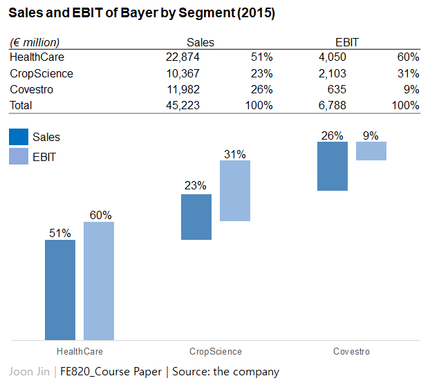
Bayer is a global chemical company with history of 150+ years founded in Germany with revenue of $60 billion in 2015.  It is well known with its signature pharmaceutical product, aspirin.  The German company had run it business with pharmaceuticals and chemicals as its major sectors until it acquired a Belgium agriculture company, Plant Genetic Systems in 2001 founding Bayer CropScience.  Bayer paid about $8 billion for Plant Genetic Systems which was the largest amount for an acquisition in Bayer’s history.  In 2016, the company defined themselves as a life science company with three major segments, pharmaceuticals, consumer-health, and crop science.  Bayer’s CropScience segment consists of crop protection and seeds, and in 2015 it represented 23% of Bayer’s net sales and 31% of earnings before interest and taxes (EBIT) as shown in Exhibit 1.  
Monsanto, an agricultural biotechnology company, was founded in 1901 but established as a sole agricultural company being divested from Pharmacia Corporation in 2000.  The US company ran its international business with revenue of $15 billion in 2015 and it represented the largest market share for seeds and crop protection products.  Its main products are glyphosate herbicide (RoundUp) and the seed products conferred the glyphosate resistance by genetic engineering (RoundUp Ready).  
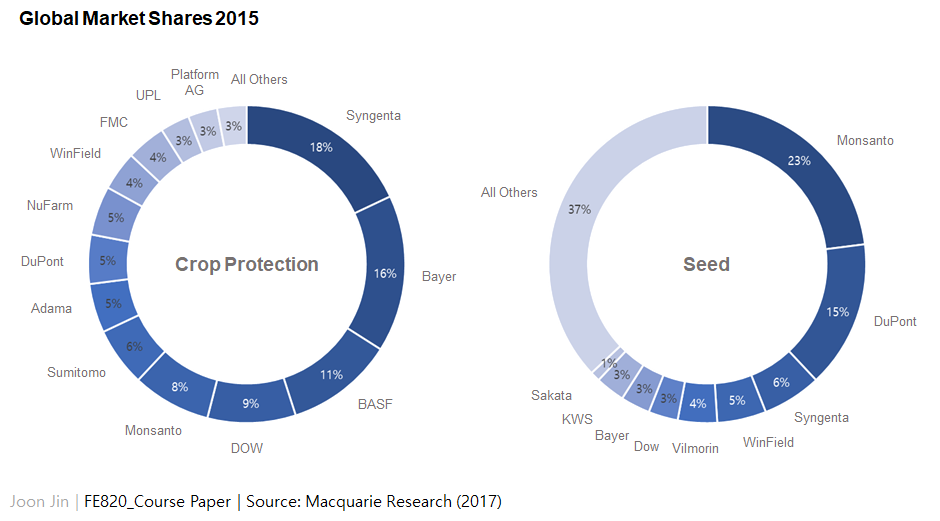
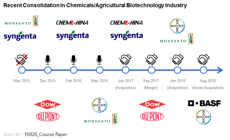
As of 2016, the agriculture industry had witnessed several major consolidations (whether or not they were successfully completed).  The industry was already dominated by a few big players (Exhibit 2), but the consolidation from 2016 occured even among the big players (Exhibit 3).  Monsanto had announced its intention to acquire Syngenta, the 3rd largest agricultural company in sales, in 2015 (although the deal was failed), Dow Chemical and DuPont announced its merger in same year which was completed in 2017, and ChemChina offered an acquisition deal to Syngenta in 2016 which was also finalized in 2017.  Amongst this drastic change in the industry, Bayer also showed its intent to acquire Monsanto in 2016 in the wake of the failure between Syngenta and Monsanto. 
The German chemical company made an unsolicited offer to buyout Monsanto in May 2016.  The initial offer price per share in May was $122 but was increased to $128 by September 2016 which is the actual price of the deal.  Bayer closed $63 billion Monsanto takeover in June 2018.  The motivation of Bayer for the acquisition might be to keep the competitors away from the largest agricultural company to secure and increase the market share in the industry.  The crop protection (chemical products such as pesticides or herbicides) had shown the strong business activity while its seeds and traits business had relatively not (Exhibit 2).  Monsanto was an appropriate company to bridge the gap since it possessed the front-running biotechnology business in agricultural industry across the world.   In addition, they were both paving ways to digital farming with data platforms and the merger could provide them with a consolidated platform.  On top of that, they were confident that the alliance between European and American companies should give them geographical merits such as diversified distribution channels, world-wide presence, and dealing with regulatory affairs in different countries.  
In this study, I valuated Monsanto as of 2016 with three different methodologies: Comparable company multiples, comparable acquisition multiples and discounted cash flow.  By doing this, I could compare the figures with the real dollar amount Bayer ended up paying, then could conclude whether or not it was in a reasonable range.

Results
Methodology 1: Comparable Company Multiples

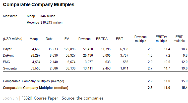
To get the comparable company multiples, I used Monsanto’s peer group companies as of the end of fiscal year 2015.  Since the agriculture industry had been consolidated by a few big chemical/biotechnology players as described above, I used four (4) companies which possessed relatively similar size in terms of sales and market capitalization with Monsanto (Exhibit 4).  The revenue multiples ranged from 1.5 and 2.7, did the EBITDA multiples from 7.2 and 14.7 and the EBIT multiples ranged from 9.8 and 19.6.  The median multiples were 2.3, 11.0 and 15.4, respectively.  The financial results from operating of Monsanto on the annual report 2015 showed the sales of $10,244 million, EBITDA of $4,310 million, and EBIT of $3,500 million.  Using those multiples and calculating the median of the enterprise values, this method came down to the business enterprise value (BEV) of  $47,280 million of Monsanto (Table 1).

Table 1. Comparable Company Multiples Analysis of Monsanto BEV 

Methodology 2: Comparable Acquisition Multiples

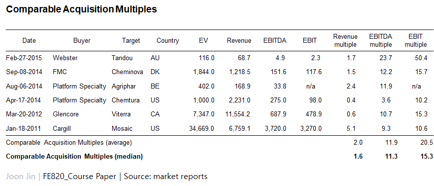
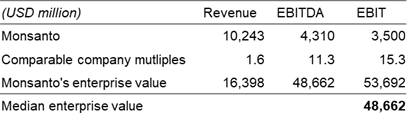
       Although the industry showed the changing landscape, there had not been many precedent acquisitions for  large target companies comparable to Monsanto before 2016.  Due to this reason, I was only able to gather acquisition data in the industry with smaller companies which could still provide an insight for Monsanto’s deal.  As seen in Exhibit 5, the revenue multiples ranged from 0.4 and 5.1, and did the EBITDA multiples from 3.6 and 23.7 and the EBIT multiples from 10.2 and 50.4.  The median multiples of revenue, EBITDA and EBIT were 1.6, 11.3 and 15.3, respectively.  Using those multiples and calculating the median of the enterprise values, Monsanto’s BEV was $48,662 million (Table 2).


Table 2. Comparable Acquisition Multiples Analysis of Monsanto BEV 


Methodology 3: Discounted Cash Flow
Discounted cash flow (DCF) is based on future estimation of a firm’s cash flow.  It uses detailed values taking specific factors into account, thus it can determine the intrinsic value of a business.  However there are significant amount of assumptions in this methodology, so assumptions should be in correct ranges to induce the right value. 
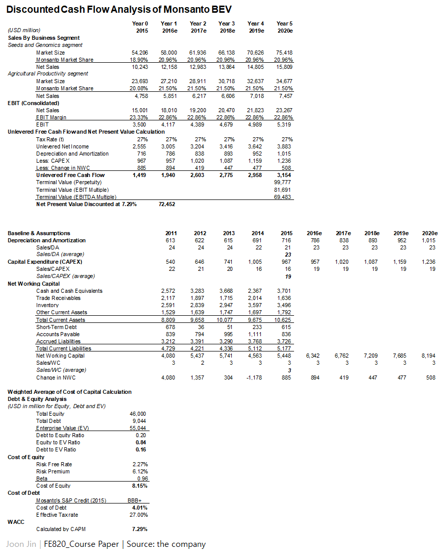
DCF method is composed of three major steps:  Estimation of free cash flow (FCF), calculation of cost of capital, and analysis of BEV.  To forecast the FCF of Monsanto, I first looked at the last five years’ earnings and cash flows of the company.  Monsanto showed $10+ billion of net sales in all years and EBIT margin ranged from 20 to 25% (Exhibit 6).  There were two business segments in Monsanto, Seeds and Genomics segment and Agricultural Productivity segment.  The former is basically a seed business, and the latter is an agricultural chemicals business selling herbicides (mostly RoundUp products).  Sales and EBIT of both segments are also shown in Exhibit 6.  To estimate the future sales and EBIT, I used those segments as baselines.  Then historical market sizes of those segments, i.e. global seed market and global herbicides market, in those years were investigated to calculate the average market shares of Monsanto in each segment (Exhibit 7, years 2011 to 2015).  Monsanto represented 20.96% and 21.50% of market shares in average in seed and herbicides fields respectively.  The market shares did not vary a lot (with standard deviations of 0.01 and 0.02) and would remain as such in the future, i.e. Monsanto’s market position would not be changed significantly as the industry was dominated with a few players and new companies were to be acquired by the players and also Monsanto kept investing in research and development constantly on top of their current competitive edges as other players.  Therefore I decided to use the average market shares in each segment to estimate the sales of Monsanto for the next five years by 2020 with the market sizes projected by reports (Research and Markets, 2017, Markets and Markets, 2017, and Transparency Market Research, 2015).  The results are shown in years 2016 to 2020 in Exhibit 7 and Exhibit 8.  Based on the sales estimation, EBIT was also forecasted.  EBIT margin was assumed to stay similar in the future as the historical EBIT margins varied in a small range.  So I used average EBIT margin of last five years which is 22.86% to forecast the next five.  With the effective income tax rate of Monsanto in 2015 which was 27%, the EBITs were utilized to calculate the unlevered net income. 
Next steps to compute the FCF for the future were estimating depreciation and amortization, capital expenditure (CAPEX), and working capital.  Since they showed even Ratio to Sales in the past, I envisioned that their investments in assets, which is in turn reflected in depreciation and amortization and CAPEX, would be grow at the same rate as sales.  This was also applied to working capital estimation based on the assumption that Monsanto had managed current assets and current liabilities roughly according to the sales.  Using all these figures based on ratio to sales with the unlevered net income, I finally resulted in the forecasted unlevered FCF of 2016 to 2020 (Exhibit 8). 
Before moving forward to have the present values in 2015 of the unlevered FCF, the terminal value beyond 2020 should be added.  In general, two methods are used to get the terminal value of a firm: Perpetuity method and Multiple method.  In perpetuity method, the terminal growth rate of 4% was used which is a nominal value of the long-term gross economic growth of the United States (source: OECD) then the terminal value derived from this method was $99,777 million.  With the discount rate which will be described below, the net present value (NPV) of Monsanto’s free cash flow and the terminal value was $80,960 million.  In multiple method, EBITDA multiple and EBITDA multiple of the comparable companies in Table 1 were multiplied by estimated EBIT in 2020 here to calculate the terminal value of the firm.  Those were $69,483 million and $81,691 million with the average value of $75,587 million.  The NPV with this terminal value represented $63,943 million.  Two NPVs were averaged into $72,452 million that is the final BEV of Monsanto using the DCF methodology (Exhibit 8).  Below is the summary of assumptions used for the DCF.

·        Sales forecast: Average of historical market shares in each segments was applied to global market size forecasted by market reports.
·        EBIT forecast: Average of historical EBIT to sales ratio was applied to forecasted sales.
·        Depreciation and Amortization, CAPEX, and NWC: Average of historical each values to sales ratio was applied to forecasted sales.
·        Terminal growth rate in Perpetuity method: The terminal growth rate of 4.0% was used which is a nominal value of the long-term gross economic growth of the United States expected by OECD.
·        Terminal value multiples in Multiple method: EBITDA multiple of 11.0 and EBIT multiple of 15.4 (in Table 1) were multiplied by estimated EBITDA and EBIT in 2020 respectively.

As described above, the discount rate was deployed here to calculate the present value of the company.  The cost of equity and cost of debt were used to compute the weighted average of cost of capital (WACC).  First, the market value of equity and debt were analyzed.  The market value of equity equals to the market capitalization and Monsanto had $46 billion of market capitalization at the end of 2015.  Per the market value of debt, the book value of debt (total of short-term and long-term debt) was used as a proxy and that was $9,044 million in 2015.  The debt to equity ratio was 20%. The ratios of equity and debt to enterprise value were 0.84 and 0.16 respectively.  
Next, the cost of equity was calculated.  The risk free rate used here is 2.27% which is the U.S. treasury bond rate in 2015. And the equity risk premium in 2015 for the S&P 500 of 6.12% was used (Damodaran, 2019).  Monsanto’s beta at the acquisition announcement was 0.96 (TheStreet, 2016).  With those figures and the capital asset pricing model (CAPM), the cost of equity of 8.15% was derived.  Next, the cost of debt was assumed with Monsanto’s credit rating. The S&P credit rating of Monsanto was BBB+ in 2015.  I was not able to obtain the bond rate of BBB+ for 2015 but the rates of BBB and A were 4.43% and 3.16% (source: YChart).  With the assumption of equal spread between ratings (I divided the difference in rates of BBB and A by three (3) as there are two grades between them: BBB+ and A-. The result value of 0.42% was used as the equal spread, then 0.42% was subtracted from BBB’s rate of 4.43% to estimate the rate of BBB+), the bond rate of BBB+ was computed and resulted in 4.01% which is the cost of debt used in this study.  Using the effective tax rate of 27% as described above and also with the weights of equity and debt, I finally derived the WACC of 7.29%.  Again, at this WACC as the discount rate, the final BEV of Monsanto using the DCF methodology represented $72,452 million.

Synergies and Final Valuation
Estimating synergies can be done with two key aspects: Cost savings and Sales synergies.  Generally it is implied that target company captures all the values from synergies thus the acquisition price would reflect it.  Baseline of this study to start is the fact that Monsanto was a giant in seeds market while Bayer was more inclined to chemical products.  According to the Bayer’s presentation to investors, they would have annual sales synergies of ~$200 million targeted as of 2022 generated from broader product portfolio and greater geographic footprint by combining sales forces and infrastructure.  Although this number represents a small portion of sales sum of both companies which was $25,000+ million in the relevant segments, I assumed there would be no synergies from sales since many of their product portfolio, e.g. target crops and target regions, were overlapped at that time and even cannibalization would be expected, so those synergies would be offset in term of sales.  Mckinsey & Company (2018) noted that three dimensions should be taken into account to estimate the sales synergies, where, how, and what to sell, but again I assumed those dimensions would be offset by the factors above then would end up with just the additive effect not the synergies. 
I rather assumed those merits would flow into the cost saving synergies.  Before beginning calculation, I took a look at the Bayer’s investor presentation and they said annual cost synergies of ~$1 billion targeted as of 2022.  When I simply applied 60% of this $1 billion to the EBIT of 2020 (as about 60~70% of $1 billion in cost savings would be achieved according to their data), the present value of $10 billion was added by the DCF method (thus up to $82 billion of BEV in DCF) .  Generally acquirors are too optimistic to estimate the positive effect of M&As, I decided not to follow this number but to estimate the cost savings on my own.  I first focused on research and development (R&D) expenses.  The accounting rules for R&D expenses are different between US GAAP and IFRS particularly with the fact that this acquisition is between the US and the European ones, but I followed US GAAP rule, i.e. all the R&D costs are regarded as expenses not assets.  As noted, Monsanto possessed strong competitiveness in crop biotechnology (and their seed products were generated from it), I expected that Bayer’s R&D on seeds would harness Monsanto’s capabilities.  Bayer CropScience had ten (10) R&D sites across the world.  Among them, five (5) sites were working on the seed research (Table 3). 


Table 3. Bayer CropScience’s  Global R&D Sites  

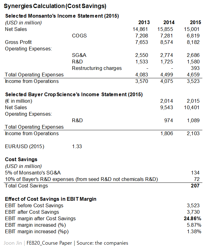
I assumed those five sites represents a half of total R&D expenses (five out of ten sites) of Bayer CropScience and could save 10% of their R&D costs following the acquisition.  Exhibit 9 shows a part of Bayer CropScience’s income statement in 2015 which was used to calculate the R&D cost savings.  In result, total annual R&D expense of $72.42 million (€54.45 million) was expected to be saved.  Another cost savings could come from selling, general and administrative expenses (SG&A).  The savings in SG&A can be achieved by reducing redundant staff members, consolidating vendors, rent savings, or merging infrastructures.  However, it was difficult to find specific data on this for the two companies, I assumed that 5% of Monsanto’s annual SG&A would be saved which was $134.3 million (Exhibit 9). 
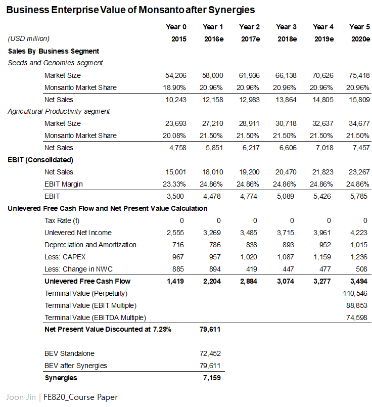
In total, about $206.72 million of annual cost savings could be achieved from R&D and SG&A, and this represented 5.9% of EBIT of Monsanto in 2015.  Therefore the EBIT margin would increased from 22.86% to 24.86%.  I applied this EBIT margin of 24.86% back to DCF to re-estimate EBITs in the future then finally the BEV of Monsanto from synergies was $79,611 million as opposed to the standalone firm’s BEV of $72,452 million.  Thus the synergies from this acquisition is $7,159 million (Exhibit 10).  Again, in this study, Monsanto was assumed to capture all the values from synergies.
Finally I calculated the common stock fair market value of Monsanto at the announcement time. Monsanto’s interest bearing debt (IBD) of $9,044 million in 2015 was subtracted from BEVs from three methodologies.  Then to derive the common stock fair market value, the synergies of $7,159 million were added to pre-discount implied equity market value from comparable company multiples and DCF methodologies, but not to comparable acquisition multiples as this methodology already implies the synergies.  Averaging the values from three methods, the final common stock fair market value was $51,860 million.  Considering the number of shares outstanding of 481.4 million, the fair market value per share ended up with the price of $108 per share (Exhibit 11, top) with the premium of 12.7% as of 2015 or 21.0% as of May 2016 (the controlling premium was ignored in this study).

Discussion and Conclusion
             The share price of $108 derived in this study is less than the actual price Bayer offered which is $122 in May 2016 then increased to $128 in September 2016.  As of one days before each announcement, the premium in May and September offers are 40% and 44%.  This discrepancy might be caused by what methodologies they used to calculate Monsanto’s value.  Now that Bayer’s patents on two top-selling drugs from HealthCare business sector were to be expired from 2023 and Bayer reportedly said the acquisition would cushion a possible drop in pharmaceutical revenues, it is probable that they relied more on DCF method valuing on earnings than the other two methods.  When I put weights for the result of DCF with 70% and 15% each for the other two methods, the value actually converged to $62,149 million in common stock fair market value and stock price of $129 per share (Exhibit 11, bottom) which is closed to the actual price of the deal (under the assumption that all the synergies to be paid to Monsanto).  Another possible cause that drew the discrepancy is the optimistic projection from Bayer for synergies.  It was difficult to see how much synergies they exactly assumed for the years in this study, but given the fact that they expected $1.2 billion in annual synergies from both sales and cost targeted as of 2022 and if this figure was reflected in the terminal value, the value of the firm would increase significantly.  
             Otherwise, it could be a dawn of big M&As in the agricultural biotechnology and chemicals field.  A partner at investment bank The Valence Group in 2017 was quoted as saying “15x EBITDA really is the new 10x.” describing recent big M&As in chemical industry.  Along with that, Bayer’s offer price actually was 15.8x EBITDA of Monsanto, and another big acquisition of the Swiss giant, Syngenta, by ChemChina in 2017 with $43 billion purchase also had the EBITDA multiple of 17.5.  Given that there had been few comparable M&As with the scale as big as Monsanto or Syngenta before 2016 and that the EBITDA multiples in this study were 11.3 (industry median), the mega trend of consolidation in this business might have been forced buyers to pay more than they had used to do.
             In 2019, in the wake of the finalization of the deal in June 2018, the media say it is one of the worst corporate deals so far (The Wall Street Journal, 2019).  Unfortunately right after the deal, glyphosate the chemical of Monsanto’s RoundUp herbicide brought pushbacks to Bayer.  Within weeks of the deal closing, Bayer lost a lawsuit alleging glyphosate causes cancer.  And the effect might have been cascaded into Bayer’s pharmaceutical business.  The consumer sentiment to a drug company, no matter what business segment is involved, could be seriously jeopardized when it comes to a safety issue.  As noted above, the deal was aimed to cushion the expiration of cash cow drugs’ patents of Bayer.  Now it turned out that the deal draws an unexpected ripple effect to the conglomerate.  It was noted above that there would be cannibalization among Monsanto’s and Bayer’s products portfolio from the acquisition in the CropScience segment.  But I did not even anticipate the negative effect would occur even against another business segment.  Nevertheless, putting aside the fact if the glyphosate allegation was transparently shared with Bayer management by Monsanto’s due diligence during the deal,  this does not mean the valuation Bayer made was significantly off target as the recent bad news are from external factors which are hard to control for the company.  We will see whether Monsanto’s value of $63 billion would pay off or not to Bayer CropScience in next few years. 

Appendix: Hindrances of Calculation
It was difficult to gather all the exact figures from public sources, so I made lots of assumptions.  For example, in the calculation of cost of debt, I used the bond rate of BBB+ based on the assumption of uniform spread between S&P ratings since I could only find the bond rates of A and BBB as described above.  Another examples are terminal growth rate and cost saving effects.  Those were especially difficult because the BEV was sensitively changed with those assumptions (see the sensitivity analysis in Exhibit 12).  With the reasonable approaches I tried and searching bunch of reports and articles for the industry, however, I made my best estimates in the study.

References
[Background Industry and Market Information]
  1. The companies’ annual reports and 10-Ks.
  2. “Nufarm: Looking for chemistry”, Macquarie Research, March 2017.
  3. “Seeds Market: Global Industry Trends, Share, Size, Growth, Opportunity and Forecast 2017-2022", Research and Markets, April 2017.
  4. “Herbicides Market by Type (Glyphosate, 2, 4-D, Diquat), Crop Type (Cereals & Grains, Oilseeds & Pulses, Fruits & Vegetables), Mode of Action (Non-selective, Selective), and Region - Global Forecast to 2022”, Markets and Markets, February 2017.
  5. “Global Herbicides Market will Continue to Expand despite Growing Demand for Organic Farming”, Transparency Market Research, November 2015.
  6. Ruth Bender, “How Bayer-Monsanto Became One of the Worst Corporate Deals—in 12 Charts”, The Wall Street Journal, August 2019.
  7. John Chartier, Alex Liu, Nikolaus Raberger and Rui Silva. “Seven Rules to Crack the Code on Revenue Synergies in M&A”,  McKinsey & Company, October 2018.
[Sources in Valuation]
  1. Damodaran, Aswath,  Equity Risk Premiums (ERP): Determinants, Estimation and Implications – The 2019 Edition (April 14, 2019). Available at SSRN: https://ssrn.com/abstract=3378246 or http://dx.doi.org/10.2139/ssrn.3378246
  2. “Monsanto (MON) Highlighted As Momo Momentum Stock”, TheStreet, May 2016.
  3. OECD: http://www.oecd.org/
  4. Macrotrends: https://www.macrotrends.net/
  5. Stockcrow: https://stockrow.com/
  6. Gurufocus: https://www.gurufocus.com/
  7. YCharts: https://ycharts.com/
  8. StreetInsider.com: https://www.streetinsider.com/

Exhibit 1.
Exhibit 2.
Exhibit 3.
Exhibit 4.
Exhibit 5.
Exhibit 6.
Exhibit 7.
Exhibit 8.
Exhibit 9.
Exhibit 10.
Exhibit 11.
Exhibit 12.