이번 글은 Corporate Finance 과목의 course paper로 한 학기 동안 진행한 프로젝트이다.
팀으로도 가능하지만 1. 친구가 없었고, 2. 경험상 그룹으로 진행하면 맡은 부분에만 집중하는 경향이 있어 전체를 아우를 수 있을 거란 기대, 3. 무엇보다 주말이라도 육아를 돕고자 조모임 왔다갔다 하는 시간을 아끼려고, 솔로팀으로 진행했다. 11개 팀 중 나 포함 두 명만 솔로팀으로 진행했다.
팀별로 지난 5년 이내의 인수건을 골라 진행하면 된다. 나는 BRIC 연재에서 몇 번 다룬 적 있는 농화학업계의 Bayer-Monsanto 건을 골랐다.
참고:
브릭연재 Bayer-Monsanto 관련 글
3개월 간 틈틈이 써왔고 지난 주말은 거의 책상에 붙어 있었다(이 글을 빌어 정말 육아에 고생이 많은 와이프님께 감사의 마음을 전한다).
리포트 전문을 옮긴다.
Caveat before reading:
1. I did not take the control premium into account. In reality, we should add the premium in a market acceptable range (e.g. 20%) on top of the business enterprise value derived from the Comparable company multiples (the control premium is already incorporated in the Comparable acquisition multiples and DCF methods). The concept is explained in another article in this blog:
http://jinjjan.blogspot.com/2019/10/mba-notecorporate-financeintroduction_29.html
2. Suggested citation: Jin, Joon Yung, "Valuation of Monsanto Acquired by Bayer", December 9, 2019. Available at
http://jinjjan.blogspot.com/2019/12/mba-case-studybayer-monsanto-acquisition.html
Valuation of Monsanto Acquired by Bayer
Dec 9th 2019
Jin, Joon Yung
Introduction
In the chemical
industry, years of 2015 to 2018 were monumental since big mergers and
acquisitions were significantly changing the landscape. Reminiscing on
their heydays back in early-mid 1990s, chemical companies sought sustainable
cash stream beyond their portfolios.
Materials for plastics and nylons had been commoditized and the market
was saturated by many players. The companies suffered from decreasing
revenues and profits in this competitive environment. Under the circumstance, most big players,
such as DuPont and BASF, already had begun to tap the agriculture business as
they saw this market was growing with various chemical applications.
Bayer is a global
chemical company with history of 150+ years founded in Germany with revenue of
$60 billion in 2015. It is well known with its
signature pharmaceutical product, aspirin. The German company had run it
business with pharmaceuticals and chemicals as its major sectors until it
acquired a Belgium agriculture company, Plant Genetic Systems in 2001 founding
Bayer CropScience. Bayer paid about $8 billion for Plant Genetic Systems
which was the largest amount for an acquisition in Bayer’s history. In 2016, the company defined themselves as a
life science company with three major segments, pharmaceuticals,
consumer-health, and crop science. Bayer’s CropScience segment consists
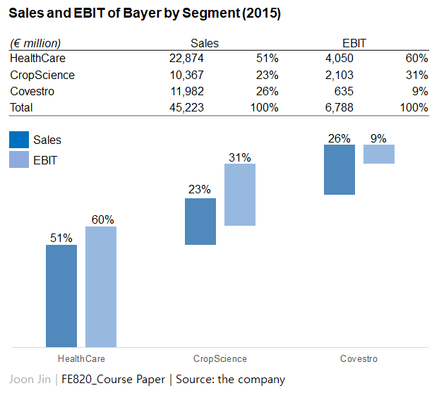
of crop protection and seeds, and in 2015 it represented 23% of Bayer’s net
sales and 31% of earnings before interest and taxes (EBIT) as shown in Exhibit
1.
Monsanto, an
agricultural biotechnology company, was founded in 1901 but established as a
sole agricultural company being divested from Pharmacia Corporation in
2000. The US company ran its international business with revenue of $15 billion in 2015 and it
represented the largest market share for seeds and crop protection
products. Its main products are glyphosate herbicide (RoundUp) and the
seed products conferred the glyphosate resistance by genetic engineering
(RoundUp Ready).
As of 2016, the
agriculture industry had witnessed several major consolidations (whether or not
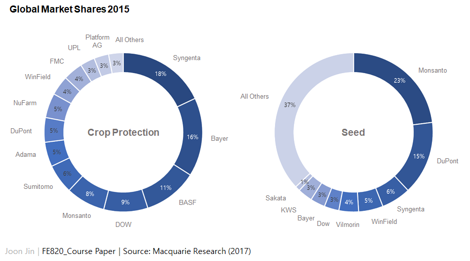
they were successfully completed). The industry was already dominated by
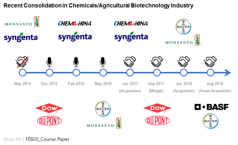
a few big players (Exhibit 2), but the consolidation from 2016 occured even
among the big players (Exhibit 3). Monsanto had announced its intention
to acquire Syngenta, the 3rd largest agricultural company in sales, in 2015
(although the deal was failed), Dow Chemical and DuPont announced its merger in
same year which was completed in 2017, and ChemChina offered an acquisition
deal to Syngenta in 2016 which was also finalized in 2017. Amongst this
drastic change in the industry, Bayer also showed its intent to acquire Monsanto
in 2016 in the wake of the failure between Syngenta and Monsanto.
The German
chemical company made an unsolicited offer to buyout Monsanto in May
2016. The initial offer price per share in May was $122 but was increased
to $128 by September 2016 which is the actual price of the deal. Bayer
closed $63 billion Monsanto takeover in June 2018. The motivation of Bayer for the acquisition
might be to keep the competitors away from the largest agricultural company to
secure and increase the market share in the industry. The crop protection
(chemical products such as pesticides or herbicides) had shown the strong
business activity while its seeds and traits business had relatively not
(Exhibit 2). Monsanto was an appropriate
company to bridge the gap since it possessed the front-running biotechnology
business in agricultural industry across the world. In addition, they
were both paving ways to digital farming with data platforms and the merger
could provide them with a consolidated platform. On top of that, they were confident that the
alliance between European and American companies should give them geographical
merits such as diversified distribution channels, world-wide presence, and
dealing with regulatory affairs in different countries.
In this study, I
valuated Monsanto as of 2016 with three different methodologies: Comparable
company multiples, comparable acquisition multiples and discounted cash
flow. By doing this, I could compare the figures with the real dollar
amount Bayer ended up paying, then could conclude whether or not it was in a
reasonable range.
Results
Methodology 1:
Comparable Company Multiples
To get the comparable company multiples, I
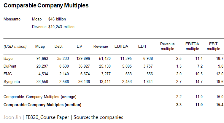
used Monsanto’s peer group companies as of the end of fiscal year 2015.
Since the agriculture industry had been consolidated by a few big
chemical/biotechnology players as described above, I used four (4) companies
which possessed relatively similar size in terms of sales and market
capitalization with Monsanto (Exhibit 4). The revenue multiples ranged
from 1.5 and 2.7, did the EBITDA multiples from 7.2 and 14.7 and the EBIT
multiples ranged from 9.8 and 19.6. The median
multiples were 2.3, 11.0 and 15.4, respectively. The financial results
from operating of Monsanto on the annual report 2015 showed the sales of
$10,244 million, EBITDA of $4,310 million, and EBIT of $3,500 million.
Using those multiples and calculating the median of the enterprise
values, this method came down to the business enterprise value (BEV) of
$47,280 million of Monsanto (Table 1).
Table 1. Comparable Company Multiples Analysis of Monsanto BEV
Methodology 2:
Comparable Acquisition Multiples
Although
the industry showed the changing landscape, there had not been many precedent
acquisitions for large target companies comparable to Monsanto before
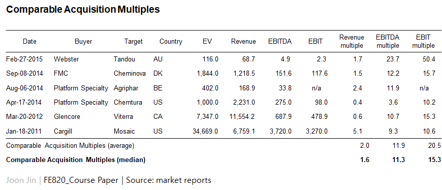
2016. Due to this reason, I was only
able to gather acquisition data in the industry with smaller companies which
could still provide an insight for Monsanto’s deal. As seen in Exhibit 5,
the revenue multiples ranged from 0.4 and 5.1, and did the EBITDA multiples
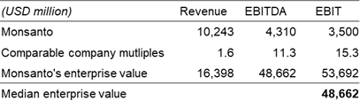
from 3.6 and 23.7 and the EBIT multiples from 10.2 and 50.4. The median multiples of revenue,
EBITDA and EBIT were 1.6, 11.3 and 15.3, respectively. Using those
multiples and calculating the median of the enterprise values,
Monsanto’s BEV was $48,662 million (Table 2).
Table 2. Comparable Acquisition Multiples Analysis of Monsanto BEV
Methodology 3:
Discounted Cash Flow
Discounted cash
flow (DCF) is based on future estimation of a firm’s cash flow. It uses
detailed values taking specific factors into account, thus it can determine the
intrinsic value of a business. However there are significant amount of
assumptions in this methodology, so assumptions should be in correct ranges to
induce the right value.
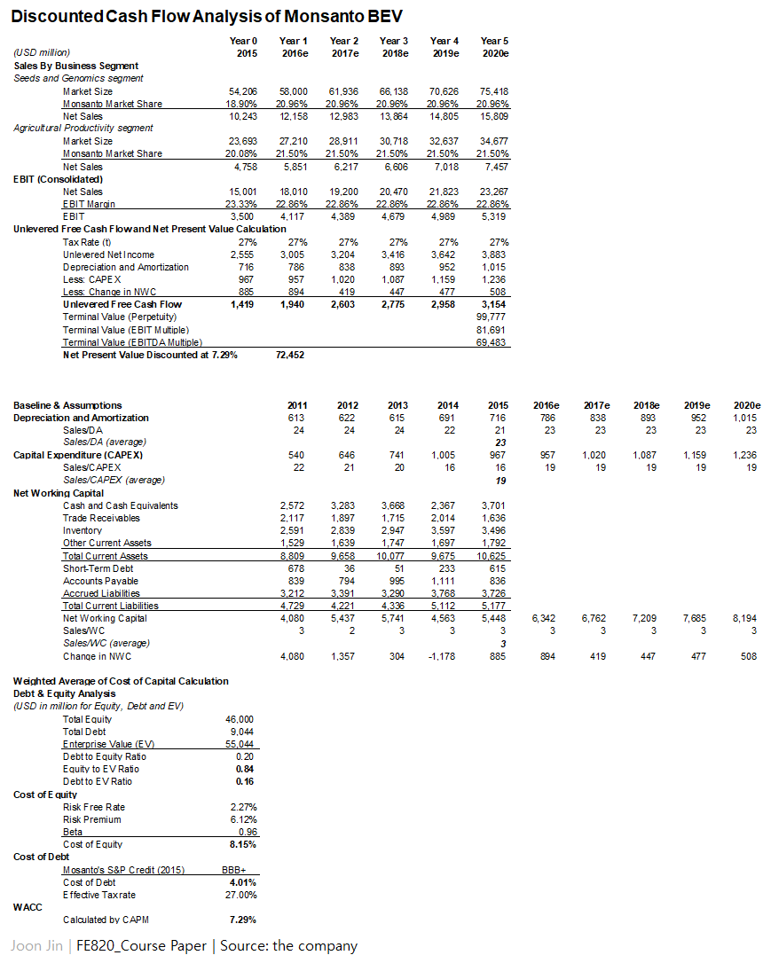
DCF method is
composed of three major steps: Estimation of free cash flow (FCF),
calculation of cost of capital, and analysis of BEV. To forecast the FCF
of Monsanto, I first looked at the last five years’ earnings and cash flows of
the company. Monsanto showed $10+ billion of net sales in all years and
EBIT margin ranged from 20 to 25% (Exhibit 6).
There were two business segments in Monsanto, Seeds and Genomics segment
and Agricultural Productivity segment. The former is basically a seed
business, and the latter is an agricultural chemicals business selling
herbicides (mostly RoundUp products).
Sales and EBIT of both segments are also shown in Exhibit 6. To estimate the future sales and EBIT, I used
those segments as baselines. Then historical market sizes of those
segments, i.e. global seed market and global herbicides market, in those years
were investigated to calculate the average market shares of Monsanto in each
segment (Exhibit 7, years 2011 to 2015).
Monsanto represented 20.96% and 21.50% of market shares in average in
seed and herbicides fields respectively. The market shares did not vary a
lot (with standard deviations of 0.01 and 0.02) and would remain as such in the
future, i.e. Monsanto’s market position would not be changed significantly as
the industry was dominated with a few players and new companies were to be
acquired by the players and also Monsanto kept investing in research and
development constantly on top of their current competitive edges as other
players. Therefore I decided to use the average market shares in each
segment to estimate the sales of Monsanto for the next five years by 2020
with the market sizes projected by reports (Research and Markets, 2017, Markets
and Markets, 2017, and Transparency Market Research, 2015). The results
are shown in years 2016 to 2020 in Exhibit 7 and Exhibit 8. Based on the sales estimation, EBIT was also
forecasted. EBIT margin was assumed to
stay similar in the future as the historical EBIT margins varied in a small
range. So I used average EBIT margin of last five years which is 22.86%
to forecast the next five. With the
effective income tax rate of Monsanto in 2015 which was 27%, the EBITs were
utilized to calculate the unlevered net income.
Next steps to
compute the FCF for the future were estimating depreciation and amortization,
capital expenditure (CAPEX), and working capital. Since they showed even
Ratio to Sales in the past, I envisioned that their investments in assets,
which is in turn reflected in depreciation and amortization and CAPEX, would be
grow at the same rate as sales. This was also applied to working capital
estimation based on the assumption that Monsanto had managed current assets and
current liabilities roughly according to the sales. Using all these figures based on ratio to
sales with the unlevered net income, I finally resulted in the forecasted
unlevered FCF of 2016 to 2020 (Exhibit 8).
Before moving
forward to have the present values in 2015 of the unlevered FCF, the terminal
value beyond 2020 should be added. In general, two methods are used to
get the terminal value of a firm: Perpetuity method and Multiple method. In perpetuity method, the terminal growth
rate of 4% was used which is a nominal value of the long-term gross
economic growth of the United States (source: OECD) then the terminal value
derived from this method was $99,777 million. With the discount rate
which will be described below, the net present value (NPV) of Monsanto’s free
cash flow and the terminal value was $80,960 million. In multiple method,
EBITDA multiple and EBITDA multiple of the comparable companies in Table 1 were
multiplied by estimated EBIT in 2020 here to calculate the terminal value of
the firm. Those were $69,483 million and $81,691 million with the average
value of $75,587 million. The NPV with
this terminal value represented $63,943 million. Two NPVs were averaged into $72,452 million
that is the final BEV of Monsanto using the DCF methodology (Exhibit 8).
Below is the summary of assumptions used for the DCF.
·
Sales forecast: Average of historical
market shares in each segments was applied to global market size forecasted by
market reports.
·
EBIT forecast: Average of historical EBIT
to sales ratio was applied to forecasted sales.
·
Depreciation and Amortization, CAPEX, and
NWC: Average of historical each values to sales ratio was applied to forecasted
sales.
·
Terminal growth rate in Perpetuity method:
The terminal growth rate of 4.0% was used which is a nominal value of
the long-term gross economic growth of the United States expected by OECD.
·
Terminal value multiples in Multiple
method: EBITDA multiple of 11.0 and EBIT multiple of 15.4 (in Table 1) were
multiplied by estimated EBITDA and EBIT in 2020 respectively.
As described above,
the discount rate was deployed here to calculate the present value of the
company. The cost of equity and cost of debt were used to compute the
weighted average of cost of capital (WACC). First, the market value of
equity and debt were analyzed. The market
value of equity equals to the market capitalization and Monsanto had $46
billion of market capitalization at the end of 2015. Per the market value
of debt, the book value of debt (total of short-term and long-term debt) was
used as a proxy and that was $9,044 million in 2015. The debt to equity ratio was 20%. The ratios
of equity and debt to enterprise value were 0.84 and 0.16
respectively.
Next, the cost of
equity was calculated. The risk free rate used here is 2.27% which is the
U.S. treasury bond rate in 2015. And the equity
risk premium in 2015 for the S&P 500 of 6.12% was used (Damodaran,
2019). Monsanto’s beta at the acquisition announcement was 0.96
(TheStreet, 2016). With those figures and the capital asset pricing model
(CAPM), the cost of equity of 8.15% was derived. Next, the cost of debt
was assumed with Monsanto’s credit rating. The S&P credit rating of
Monsanto was BBB+ in 2015. I was not able to obtain the bond rate of BBB+
for 2015 but the rates of BBB and A were 4.43% and 3.16% (source:
YChart). With the assumption of equal spread between ratings (I divided
the difference in rates of BBB and A by three (3) as there are two grades
between them: BBB+ and A-. The result value of 0.42% was used as the equal
spread, then 0.42% was subtracted from BBB’s rate of 4.43% to estimate the rate
of BBB+), the bond rate of BBB+ was computed and resulted in 4.01% which is the
cost of debt used in this study. Using the effective tax rate of 27% as
described above and also with the weights of equity and debt, I finally derived
the WACC of 7.29%. Again, at this WACC
as the discount rate, the final BEV of Monsanto using the DCF methodology
represented $72,452 million.
Synergies and
Final Valuation
Estimating
synergies can be done with two key aspects: Cost savings and Sales
synergies. Generally it is implied that target company captures all the
values from synergies thus the acquisition price would reflect it.
Baseline of this study to start is the fact that Monsanto was a giant in seeds
market while Bayer was more inclined to chemical products. According to
the Bayer’s presentation to investors, they would have annual sales synergies
of ~$200 million targeted as of 2022 generated from broader product portfolio
and greater geographic footprint by combining sales forces and
infrastructure. Although this number represents a small portion of sales
sum of both companies which was $25,000+ million in the relevant segments, I
assumed there would be no synergies from sales since many of their product
portfolio, e.g. target crops and target regions, were overlapped at that time
and even cannibalization would be expected, so those synergies would be offset
in term of sales. Mckinsey & Company (2018) noted that three
dimensions should be taken into account to estimate the sales synergies, where,
how, and what to sell, but again I assumed those dimensions would be offset by
the factors above then would end up with just the additive effect not the
synergies.
I rather assumed
those merits would flow into the cost saving synergies. Before beginning
calculation, I took a look at the Bayer’s investor presentation and they said
annual cost synergies of ~$1 billion targeted as of 2022. When I simply
applied 60% of this $1 billion to the EBIT of 2020 (as about 60~70% of $1
billion in cost savings would be achieved according to their data), the present
value of $10 billion was added by the DCF method (thus up to $82 billion of BEV
in DCF) . Generally acquirors are too optimistic to estimate the positive
effect of M&As, I decided not to follow this number but to estimate the
cost savings on my own. I first focused
on research and development (R&D) expenses.
The accounting rules for R&D expenses are different between US GAAP
and IFRS particularly with the fact that this acquisition is between the US and
the European ones, but I followed US GAAP rule, i.e. all the R&D costs are
regarded as expenses not assets. As noted, Monsanto possessed strong
competitiveness in crop biotechnology (and their seed products were generated
from it), I expected that Bayer’s R&D on seeds would harness Monsanto’s
capabilities. Bayer CropScience had ten
(10) R&D sites across the world.
Among them, five (5) sites were working on the seed research (Table
3).
Table 3. Bayer CropScience’s Global R&D Sites
I assumed those
five sites represents a half of total R&D expenses (five out of ten sites)
of Bayer CropScience and could save 10% of their R&D costs following the
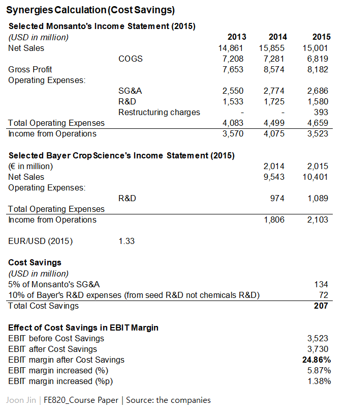
acquisition. Exhibit 9 shows a part of Bayer CropScience’s income
statement in 2015 which was used to calculate the R&D cost savings. In result, total annual R&D expense of
$72.42 million (€54.45 million) was expected to
be saved. Another cost savings could come from selling, general and
administrative expenses (SG&A). The savings in SG&A can be
achieved by reducing redundant staff members, consolidating vendors, rent
savings, or merging infrastructures. However, it was difficult to find
specific data on this for the two companies, I assumed that 5% of Monsanto’s
annual SG&A would be saved which was $134.3 million (Exhibit 9).
In
total, about $206.72 million of annual cost savings could be achieved from
R&D and SG&A, and this represented 5.9% of EBIT of Monsanto in
2015. Therefore the EBIT margin would increased from 22.86% to
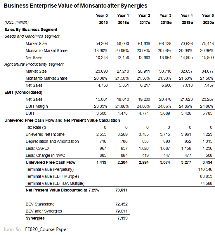
24.86%. I applied this EBIT margin of
24.86% back to DCF to re-estimate EBITs in the future then finally the BEV of
Monsanto from synergies was $79,611 million as opposed to the standalone firm’s
BEV of $72,452 million. Thus the synergies from this acquisition is
$7,159 million (Exhibit 10). Again, in this
study, Monsanto was assumed to capture all the values from synergies.
Finally I
calculated the common stock fair market value of Monsanto at the announcement
time. Monsanto’s interest bearing debt (IBD) of $9,044 million in 2015 was
subtracted from BEVs from three methodologies. Then to derive the common
stock fair market value, the synergies of $7,159 million were added to
pre-discount implied equity market value from comparable company multiples and
DCF methodologies, but not to comparable acquisition multiples as this
methodology already implies the synergies. Averaging the values from
three methods, the final common stock fair market value was $51,860
million. Considering the number of
shares outstanding of 481.4 million, the fair market value per share ended up
with the price of $108 per share (Exhibit 11, top) with the premium of 12.7% as
of 2015 or 21.0% as of May 2016 (the controlling premium was ignored in this
study).
Discussion and
Conclusion
The share price of $108 derived in
this study is less than the actual price Bayer offered which is $122 in May
2016 then increased to $128 in September 2016. As of one days before each
announcement, the premium in May and September offers are 40% and 44%. This discrepancy might be caused by what
methodologies they used to calculate Monsanto’s value. Now that Bayer’s
patents on two top-selling drugs from HealthCare business sector were to be expired
from 2023 and Bayer reportedly said the acquisition would cushion a possible
drop in pharmaceutical revenues, it is probable that they relied more on DCF
method valuing on earnings than the other two methods. When I put weights
for the result of DCF with 70% and 15% each for the other two methods, the
value actually converged to $62,149 million in common stock fair market value
and stock price of $129 per share (Exhibit 11, bottom) which is closed to the
actual price of the deal (under the assumption that all the synergies to be
paid to Monsanto). Another possible cause that drew the discrepancy is
the optimistic projection from Bayer for synergies. It was difficult to see how much synergies
they exactly assumed for the years in this study, but given the fact that they
expected $1.2 billion in annual synergies from both sales and cost targeted as
of 2022 and if this figure was reflected in the terminal value, the value of
the firm would increase significantly.
Otherwise, it could be a dawn of
big M&As in the agricultural biotechnology and chemicals field. A
partner at investment bank The Valence Group in 2017 was quoted as saying “15x
EBITDA really is the new 10x.” describing recent big M&As in chemical
industry. Along with that, Bayer’s offer price actually was 15.8x EBITDA
of Monsanto, and another big acquisition of the Swiss giant, Syngenta, by
ChemChina in 2017 with $43 billion purchase also had the EBITDA multiple of
17.5. Given that there had been few comparable M&As with the scale as
big as Monsanto or Syngenta before 2016 and that the EBITDA multiples in this
study were 11.3 (industry median), the mega trend of consolidation in this
business might have been forced buyers to pay more than they had used to do.
In 2019, in the wake of the finalization
of the deal in June 2018, the media say it is one of the worst corporate deals
so far (The Wall Street Journal, 2019). Unfortunately right after the
deal, glyphosate the chemical of Monsanto’s RoundUp herbicide brought pushbacks
to Bayer. Within weeks of the deal
closing, Bayer lost a lawsuit alleging glyphosate causes cancer. And the
effect might have been cascaded into Bayer’s pharmaceutical business. The consumer sentiment to a drug company, no matter
what business segment is involved, could be seriously jeopardized when it comes
to a safety issue. As noted above, the deal was aimed to cushion the
expiration of cash cow drugs’ patents of Bayer.
Now it turned out that the deal draws an unexpected ripple effect to the
conglomerate. It was noted above that
there would be cannibalization among Monsanto’s and Bayer’s products portfolio
from the acquisition in the CropScience segment. But I did not even
anticipate the negative effect would occur even against another business
segment. Nevertheless, putting aside the
fact if the glyphosate allegation was transparently shared with Bayer
management by Monsanto’s due diligence during the deal, this does not mean the valuation Bayer made
was significantly off target as the recent bad news are from external factors
which are hard to control for the company. We will see whether Monsanto’s
value of $63 billion would pay off or not to Bayer CropScience in next few
years.
Appendix:
Hindrances of Calculation
It was difficult
to gather all the exact figures from public sources, so I made lots of
assumptions. For example, in the calculation of cost of debt, I used the
bond rate of BBB+ based on the assumption of uniform spread between S&P
ratings since I could only find the bond rates of A and BBB as described
above. Another examples are terminal growth rate and cost saving
effects. Those were especially difficult
because the BEV was sensitively changed with those assumptions (see the
sensitivity analysis in Exhibit 12).
With the reasonable approaches I tried and searching bunch of reports
and articles for the industry, however, I made my best estimates in the study.
References
[Background
Industry and Market Information]
- The companies’ annual
reports and 10-Ks.
- “Nufarm: Looking for
chemistry”, Macquarie Research, March 2017.
- “Seeds Market: Global
Industry Trends, Share, Size, Growth, Opportunity and Forecast
2017-2022", Research and Markets, April 2017.
- “Herbicides Market by
Type (Glyphosate, 2, 4-D, Diquat), Crop Type (Cereals & Grains,
Oilseeds & Pulses, Fruits & Vegetables), Mode of Action
(Non-selective, Selective), and Region - Global Forecast to 2022”, Markets
and Markets, February 2017.
- “Global Herbicides Market
will Continue to Expand despite Growing Demand for Organic Farming”, Transparency
Market Research, November 2015.
- Ruth Bender, “How
Bayer-Monsanto Became One of the Worst Corporate Deals—in 12 Charts”, The
Wall Street Journal, August 2019.
- John Chartier, Alex Liu,
Nikolaus Raberger and Rui Silva. “Seven Rules to Crack the Code on Revenue
Synergies in M&A”, McKinsey & Company, October 2018.
[Sources in
Valuation]
- Damodaran, Aswath, Equity
Risk Premiums (ERP): Determinants, Estimation and Implications – The 2019
Edition (April 14, 2019). Available at SSRN: https://ssrn.com/abstract=3378246
or http://dx.doi.org/10.2139/ssrn.3378246
- “Monsanto (MON)
Highlighted As Momo Momentum Stock”, TheStreet, May 2016.
- OECD: http://www.oecd.org/
- Macrotrends: https://www.macrotrends.net/
- Stockcrow: https://stockrow.com/
- Gurufocus: https://www.gurufocus.com/
- YCharts: https://ycharts.com/
- StreetInsider.com: https://www.streetinsider.com/
Exhibit 1.
Exhibit 2.
Exhibit 3.
Exhibit 4.
Exhibit 5.
Exhibit 6.
Exhibit 7.
Exhibit 8.
Exhibit 9.
Exhibit 10.
Exhibit 11.
Exhibit 12.